2. Getting Started¶

Here, we explain how to use ABCpy to quntify parameter uncertainty of a probabbilistic model given some observed dataset. If you are new to uncertainty quantification using Approximate Bayesian Computation (ABC), we recommend you to start with the Parameters as Random Variables section.

Parameters as Random Variables¶

As an example, if we have measurements of the height of a group of grown up human and it is also known that a Gaussian distribution is an appropriate probabilistic model for these kind of observations, then our observed dataset would be measurement of heights and the probabilistic model would be Gaussian.

height_obs = [160.82499176, 167.24266737, 185.71695756, 153.7045709, 163.40568812, 140.70658699, 169.59102084, 172.81041696, 187.38782738, 179.66358934, 176.63417241, 189.16082803, 181.98288443, 170.18565017, 183.78493886, 166.58387299, 161.9521899, 155.69213073, 156.17867343, 144.51580379, 170.29847515, 197.96767899, 153.36646527, 162.22710198, 158.70012047, 178.53470703, 170.77697743, 164.31392633, 165.88595994, 177.38083686, 146.67058471763457, 179.41946565658628, 238.02751620619537, 206.22458790620766, 220.89530574344568, 221.04082532837026, 142.25301427453394, 261.37656571434275, 171.63761180867033, 210.28121820385866, 237.29130237612236, 175.75558340169619, 224.54340549862235, 197.42448680731226, 165.88273684581381, 166.55094082844519, 229.54308602661584, 222.99844054358519, 185.30223966014586, 152.69149367593846, 206.94372818527413, 256.35498655339154, 165.43140916577741, 250.19273595481803, 148.87781549665536, 223.05547559193792, 230.03418198709608, 146.13611923127021, 138.24716809523139, 179.26755740864527, 141.21704876815426, 170.89587081800852, 222.96391329259626, 188.27229523693822, 202.67075179617672, 211.75963110985992, 217.45423324370509]

The Gaussian or Normal model has two parameters: the mean, denoted by \(\mu\), and the standard deviation, denoted by \(\sigma\). We consider these parameters as random variables. The goal of ABC is to quantify the uncertainty of these parameters from the information contained in the observed data.

In ABCpy, a abcpy.probabilisticmodels.ProbabilisticModel object represents probabilistic relationship between random variables or between random variables and observed data. Each of the ProbabilisticModel object has a number of input parameters: they are either random variables (output of another ProbabilisticModel object) or constant values and considered known to the user (Hyperparameters). If you are interested in implementing your own probabilistic model, please check the implementing a new model section.

To define a parameter of a model as a random variable, you start by assigning a prior distribution on them. We can utilize prior knowledge about these parameters as prior distribution. In the absence of prior knowledge, we still need to provide prior information and a non-informative flat disribution on the parameter space can be used. The prior distribution on the random variables are assigned by a probabilistic model which can take other random variables or hyper parameters as input.

In our Gaussian example, providing prior information is quite simple. We know from experience that the average height should be somewhere between 150cm and 200cm, while the standard deviation is around 5 to 25. In code, this would look as follows:

from abcpy.continuousmodels import Uniform
mu = Uniform([[150], [200]], )
sigma = Uniform([[5], [25]], )
# define the model
height = Gaussian([mu, sigma], name='height')

We have defined the parameter \(\mu\) and \(\sigma\) of the Gaussian model as random variables and assigned Uniform prior distributions on them. The parameters of the prior distribution \((150, 200, 5, 25)\) are assumed to be known to the user, hence they are called hyperparameters. Also, internally, the hyperparameters are converted to Hyperparameter objects. Note that you are also required to pass a name string while defining a random variable. In the final output, you will see these names, together with the relevant outputs corresponding to them.

For uncertainty quantification, we follow the philosophy of Bayesian inference. We are interested in the distribution of the parameters we get after incorporating the information that is implicit in the observed dataset with the prior information. This target distribution is called posterior distribution of the parameters. For inference, we draw independent and identical sample values from the posterior distribution. These sampled values are called posterior samples and used to either approximate the posterior distribution or to integrate in a Monte Carlo style w.r.t the posterior distribution. The posterior samples are the ones you get as a result of applying an ABC inference scheme.

The heart of the ABC inferential algorithm is a measure of discrepancy between the observed dataset and the synthetic dataset (simulated/generated from the model). Often, computation of discrepancy measure between the observed and synthetic dataset is not feasible (e.g., high dimensionality of dataset, computationally to complex) and the discrepancy measure is defined by computing a distance between relevant summary statistics extracted from the datasets. Here we first define a way to extract summary statistics from the dataset.

from abcpy.statistics import Identity
statistics_calculator = Identity(degree = 2, cross = False)

Next we define the discrepancy measure between the datasets, by defining a distance function (LogReg distance is chosen here) between the extracted summary statistics. If we want to define the discrepancy measure through a distance function between the datasets directly, we choose Identity as summary statistics which gives the original dataset as the extracted summary statistics. This essentially means that the distance object automatically extracts the statistics from the datasets, and then compute the distance between the two statistics.

from abcpy.distances import LogReg
distance_calculator = LogReg(statistics_calculator)

Algorithms in ABCpy often require a perturbation kernel, a tool to explore the parameter space. Here, we use the default kernel provided, which explores the parameter space of random variables, by using e.g. a multivariate Gaussian distribution or by performing a random walk depending on whether the corresponding random variable is continuous or discrete. For a more involved example, please consult Complex Perturbation Kernels.

from abcpy.perturbationkernel import DefaultKernel
kernel = DefaultKernel([mu, sigma])

Finally, we need to specify a backend that determins the parallelization framework to use. The example code here uses the dummy backend BackendDummy which does not parallelize the computation of the inference schemes, but which this is handy for prototyping and testing. For more advanced parallelization backends available in ABCpy, please consult Using Parallelization Backends section.

from abcpy.backends import BackendDummy as Backend
backend = Backend()

In this example, we choose PMCABC algorithm (inference scheme) to draw posterior samples of the parameters. Therefore, we instantiate a PMCABC object by passing the random variable corresponding to the observed dataset, the distance function, backend object, perturbation kernel and a seed for the random number generator.

# define sampling scheme
from abcpy.inferences import PMCABC
sampler = PMCABC([height], [distance_calculator], backend, kernel, seed=1)

Finally, we can parametrize the sampler and start sampling from the posterior distribution of the parameters given the observed dataset:

# sample from scheme
T, n_sample, n_samples_per_param = 3, 250, 10
eps_arr = np.array([.75])
epsilon_percentile = 10
journal = sampler.sample([height_obs],  T, eps_arr, n_sample, n_samples_per_param, epsilon_percentile)

The above inference scheme gives us samples from the posterior distribution of the parameter of interest height quantifying the uncertainty of the inferred parameter, which are stored in the journal object. See Post Analysis for further information on extracting results.

Note that the model and the observations are given as a list. This is due to the fact that in ABCpy, it is possible to have hierarchical models, building relationships between co-occuring groups of datasets. To learn more, see the Hierarchical Model section.

The full source can be found in examples/extensions/models/gaussian_python/pmcabc_gaussian_model_simple.py. To execute the code you only need to run

python3 pmcabc_gaussian_model_simple.py

Probabilistic Dependency between Random Variables¶

Since release 0.5.0 of ABCpy, a probabilistic dependency structures (e.g., a Bayesian network) between random variables can be modelled. Behind the scene, ABCpy will represent this dependency structure as a directed acyclic graph (DAG) such that the inference can be done on the full graph. Further we can also define new random variables through operations between existing random variables. To make this concept more approachable, we now exemplify an inference problem on a probabilistic dependency structure.

Let us consider the following example: Assume we have a school with different classes. Each class has some number of students. All students of the school take an exam and receive some grade. Lets consider the grades of the students as our observed dataset:

The grades of the students depend on several variables: if there were bias, the size of the class a student is in, as well as the social background of the student. The dependency structure between these variables can be defined using the following Bayesian network:

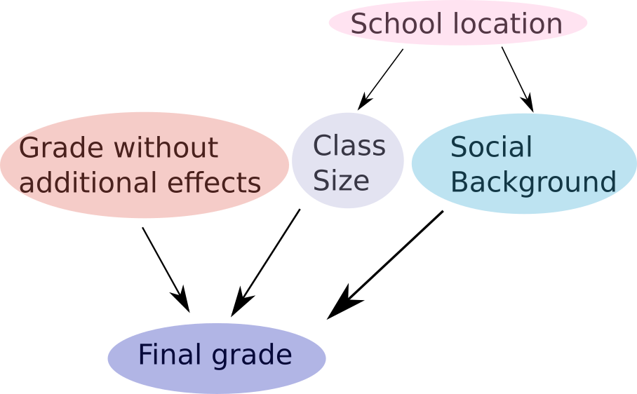
Here we assume the size of a class the student belongs to and his/her social background are normally distributed with some mean and variance. However, they also both depend on the location of the school. In certain neighbourhoods, the class size might be larger, or the social background might differ. We therefore have additional parameters, specifying the mean of these normal distributions will vary uniformly between some lower and upper bounds. Finally, we can assume that the grade without any bias would be a normally distributed parameter around an average grade.

We can define these random variables and the dependencies between them (in a nutshell, a Bayesian network) in ABCpy in the following way:

So, each student will receive some grade without additional effects which is normally distributed, but then the final grade recieved will be a function of grade without additional effects and the other random variables defined beforehand (e.g., school_location, class_size and background). The model for the final grade of the students now can be written as:

Notice here we created a new random variable final_grade, by subtracting the random variables class_size and background from the random variable grade. In short, this illustrates that you can perform standard operations “+”, “-“, “*”, “/” and “**” (the power operator in Python) on any two random variables, to get a new random variable. It is possible to perform these operations between two random variables additionally to the general data types of Python (integer, float, and so on) since they are converted to HyperParameters.

Please keep in mind that parameters defined via operations will not be included in your list of parameters in the journal file. However, all parameters that are part of the operation, and are not fixed, will be included, so you can easily perform the required operations on the final result to get these parameters, if necessary. In addition, you can now also use the [] operator (the access operator in Python). This allows you to select single values or ranges of a multidimensional random variable as a parameter of a new random variable.

To do inference on the Baysian network given the observed datat, we again have to define some summary statistics of our data (similar to the Parameters as Random Variables section).

And just as before, we need to provide a distance measure, a backend and a kernel to the inference scheme of our choice, which again is PMCABC.

Finally, we can parametrize the sampler and start sampling from the posterior distribution:

The source code can be found in examples/hierarchicalmodels/pmcabc_inference_on_single_set_of_obs.py and can be run as show above.

Hierarchical Model¶

As mentioned above, ABCpy supports inference on hierarchical models. Hierarchical models can share some of the parameters of interest and model co-occuring datasets. To illustrate how this is implemented, we will follow the example model given in Probabilistic Dependency between Random Variables section and extend it to co-occuring datasets.

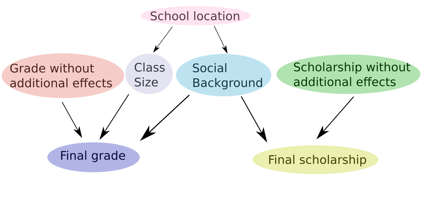
Let us assume that in addition to the final grade of a student, we have (co-occuring, observed) data for final scholarships given out by the school to the students. Whether a student gets a scholarship depends on his social background and on an independent score.

scholarship_obs = [2.7179657436207805, 2.124647285937229, 3.07193407853297, 2.335024761813643, 2.871893855192, 3.4332002458233837, 3.649996835818173, 3.50292335102711, 2.815638168018455, 2.3581613289315992, 2.2794821846395568, 2.8725835459926503, 3.5588573782815685, 2.26053126526137, 1.8998143530749971, 2.101110815311782, 2.3482974964831573, 2.2707679029919206, 2.4624550491079225, 2.867017757972507, 3.204249152084959, 2.4489542437714213, 1.875415915801106, 2.5604889644872433, 3.891985093269989, 2.7233633223405205, 2.2861070389383533, 2.9758813233490082, 3.1183403287267755, 2.911814060853062, 2.60896794303205, 3.5717098647480316, 3.3355752461779824, 1.99172284546858, 2.339937680892163, 2.9835630207301636, 2.1684912355975774, 3.014847335983034, 2.7844122961916202, 2.752119871525148, 2.1567428931391635, 2.5803629307680644, 2.7326646074552103, 2.559237193255186, 3.13478196958166, 2.388760269933492, 3.2822443541491815, 2.0114405441787437, 3.0380056368041073, 2.4889680313769724, 2.821660164621084, 3.343985964873723, 3.1866861970287808, 4.4535037154856045, 3.0026333138006027, 2.0675706089352612, 2.3835301730913185, 2.584208398359566, 3.288077633446465, 2.6955853384148183, 2.918315169739928, 3.2464814419322985, 2.1601516779909433, 3.231003347780546, 1.0893224045062178, 0.8032302688764734, 2.868438615047827]

We assume the score is normally distributed and we model it as follows:

scholarship_without_additional_effects = Normal([[2], [0.5]], )

We model the impact of the students social background on the scholarship as follows:

final_scholarship = scholarship_without_additional_effects + 3*background

With this we now have two root ProbabilisicModels (random variables), namely final_grade and final_scholarship, whose output can directly compared to the observed datasets grade_obs and scholarship_obs. With this we are able to do an inference computation on all free parameters of the hierarchical model (of the DAG) given our observations.

To inference uncertainty of our parameters, we follow the same steps as in our previous examples: We choose summary statistics, distance, inference scheme, backend and kernel. We will skip the definitions that have not changed from the previous section. However, we would like to point out the difference in definition of the distance. Since we are now considering two observed datasets, we need to define an distances on them separately. Here, we use the Euclidean distance for each observed data set and corresponding simulated dataset. You can use two different distances on two different observed datasets.

# Define a summary statistics for final grade and final scholarship
from abcpy.statistics import Identity
statistics_calculator_final_grade = Identity(degree = 2, cross = False)
statistics_calculator_final_scholarship = Identity(degree = 3, cross = False)

# Define a distance measure for final grade and final scholarship
from abcpy.distances import Euclidean
distance_calculator_final_grade = Euclidean(statistics_calculator_final_grade)
distance_calculator_final_scholarship = Euclidean(statistics_calculator_final_scholarship)

Using these two distance functions with the final code look as follows:

# Define a backend
from abcpy.backends import BackendDummy as Backend
backend = Backend()

# Define a perturbation kernel
from abcpy.perturbationkernel import DefaultKernel
kernel = DefaultKernel([school_location, class_size, grade_without_additional_effects, \
                        background, scholarship_without_additional_effects])

# Define sampling parameters
T, n_sample, n_samples_per_param = 3, 250, 10
eps_arr = np.array([.75])
epsilon_percentile = 10

# Define sampler
from abcpy.inferences import PMCABC
sampler = PMCABC([final_grade, final_scholarship], \
                 [distance_calculator_final_grade, distance_calculator_final_scholarship], backend, kernel)

# Sample
journal = sampler.sample([grades_obs, scholarship_obs], \
                         T, eps_arr, n_sample, n_samples_per_param, epsilon_percentile)

Observe that the lists given to the sampler and the sampling method now contain two entries. These correspond to the two different observed data sets respectively. Also notice now we provide two different distances corresponding to the two different root models and their observed datasets. Presently ABCpy combines the distances by a linear combination, however customized combination strategies can be implemented by the user.

The full source code can be found in examples/hierarchicalmodels/pmcabc_inference_on_multiple_sets_of_obs.py.

Complex Perturbation Kernels¶

As pointed out earlier, it is possible to define complex perturbation kernels, perturbing different random variables in different ways. Let us take the same example as in the Hierarchical Model and assume that we want to perturb the schools location as well as the scholarship score, using a multivariate normal kernel. However, the remaining parameters we would like to perturb using a multivariate Student’s-T kernel. This can be implemented as follows:

from abcpy.perturbationkernel import MultivariateNormalKernel, MultivariateStudentTKernel
kernel_1 = MultivariateNormalKernel([school_location, scholarship])
kernel_2 = MultivariateStudentTKernel([class_size, background, grade], df=3)

We have now defined how each set of parameters is perturbed on its own. The sampler object, however, needs to be provided with one single kernel. We, therefore, provide a class which groups the above kernels together. This class, abcpy.perturbationkernel.JointPerturbationKernel, knows how to perturb each set of parameters individually. It just needs to be provided with all the relevant kernels:

from abcpy.perturbationkernel import JointPerturbationKernel
kernel = JointPerturbationKernel([kernel_1, kernel_2])

This is all that needs to be changed. The rest of the implementation works the exact same as in the previous example. If you would like to implement your own perturbation kernel, please check Implementing a new Perturbation Kernel. Please keep in mind that you can only perturb parameters. You cannot use the access operator to perturb one component of a multi-dimensional random variable differently than another component of the same variable.

The source code to this section can be found in examples/extensions/perturbationkernels/pmcabc_perturbation_kernels.py

Inference Schemes¶

In ABCpy, we implement widely used and advanced variants of ABC inferential schemes:

Rejection ABC abcpy.inferences.RejectionABC,
Population Monte Carlo ABC abcpy.inferences.PMCABC,
Sequential Monte Carlo ABC abcpy.inferences.SMCABC,
Replenishment sequential Monte Carlo ABC (RSMC-ABC) abcpy.inferences.RSMCABC,
Adaptive population Monte Carlo ABC (APMC-ABC) abcpy.inferences.APMCABC,
ABC with subset simulation (ABCsubsim) abcpy.inferences.ABCsubsim, and
Simulated annealing ABC (SABC) abcpy.inferences.SABC.

To perform ABC algorithms, we provide different standard distance functions between datasets, e.g., a discrepancy measured by achievable classification accuracy between two datasets

abcpy.distances.Euclidean,
abcpy.distances.LogReg,
abcpy.distances.PenLogReg.

We also have implemented the population Monte Carlo abcpy.inferences.PMC algorithm to infer parameters when the likelihood or approximate likelihood function is available. For approximation of the likelihood function we provide two methods:

Synthetic likelihood approximation abcpy.approx_lhd.SynLiklihood, and another method using
penalized logistic regression abcpy.approx_lhd.PenLogReg.

Next we explain how we can use PMC algorithm using approximation of the likelihood functions. As we are now considering two observed datasets corresponding to two root models, we need to define an approximation of likelihood function for each of them separately. Here, we use the abcpy.approx_lhd.SynLiklihood for each of the root models. It is also possible to use two different approximate likelihoods for two different root models.

# Define a summary statistics for final grade and final scholarship
from abcpy.statistics import Identity
statistics_calculator_final_grade = Identity(degree = 2, cross = False)
statistics_calculator_final_scholarship = Identity(degree = 3, cross = False)

# Define a distance measure for final grade and final scholarship
from abcpy.approx_lhd import SynLiklihood
approx_lhd_final_grade = SynLiklihood(statistics_calculator_final_grade)
approx_lhd_final_scholarship = SynLiklihood(statistics_calculator_final_scholarship)

We then parametrize the sampler and sample from the posterior distribution.

# Define sampling parameters
T, n_sample, n_samples_per_param = 3, 250, 10

# Define sampler
from abcpy.inferences import PMC
sampler = PMC([final_grade, final_scholarship], \
                 [approx_lhd_final_grade, approx_lhd_final_scholarship], backend, kernel)

# Sample
journal = sampler.sample([grades_obs, scholarship_obs], T, n_sample, n_samples_per_param)


analyse_journal(journal):

Observe that the lists given to the sampler and the sampling method now contain two entries. These correspond to the two different observed data sets respectively. Also notice now we provide two different distances corresponding to the two different root models and their observed datasets. Presently ABCpy combines the distances by a linear combination. Further possibilities of combination will be made available in later versions of ABCpy.

The source code can be found in examples/approx_lhd/pmc_hierarchical_models.py.

Summary Selection¶

We have noticed in the Parameters as Random Variables Section, the discrepancy measure between two datasets is defined by a distance function between extracted summary statistics from the datasets. Hence, the ABC algorithms are subjective to the summary statistics choice. This subjectivity can be avoided by a data-driven summary statistics choice from the available summary statistics of the dataset. In ABCpy we provide a semi-automatic summary selection procedure in abcpy.summaryselections.Semiautomatic

Taking our initial example from Parameters as Random Variables where we model the height of humans, we can had summary statistics defined as follows:

# define statistics
from abcpy.statistics import Identity
statistics_calculator = Identity(degree = 3, cross = True)

Then we can learn the optimized summary statistics from the given list of summary statistics using the semi-automatic summary selection procedure as following:

# Learn the optimal summary statistics using Semiautomatic summary selection
from abcpy.summaryselections import Semiautomatic
summary_selection = Semiautomatic([height], statistics_calculator, backend,
                                  n_samples=1000,n_samples_per_param=1, seed=1)

# Redefine the statistics function
statistics_calculator.statistics = lambda x, f2=summary_selection.transformation, \
                                          f1=statistics_calculator.statistics: f2(f1(x))

Then we can perform the inference as before, but the distances will be computed on the newly learned summary statistics using the semi-automatic summary selection procedure.

Model Selection¶

A further extension of the inferential problem is the selection of a model (M), given an observed dataset, from a set of possible models. The package also includes a parallelized version of random forest ensemble model selection algorithm [abcpy.modelselections.RandomForest].

Lets consider an array of two models Normal and StudentT. We want to find out which one of these two models are the most suitable one for the observed dataset y_obs.

## Create a array of models
from abcpy.continuousmodels import Uniform, Normal, StudentT
model_array = [None]*2

#Model 1: Gaussian
mu1 = Uniform([[150], [200]], name='mu1')
sigma1 = Uniform([[5.0], [25.0]], name='sigma1')
model_array[0] = Normal([mu1, sigma1])

#Model 2: Student t
mu2 = Uniform([[150], [200]], name='mu2')
sigma2 = Uniform([[1], [30.0]], name='sigma2')
model_array[1] = StudentT([mu2, sigma2])

We first need to initiate the Model Selection scheme, for which we need to define the summary statistics and backend:

# define statistics
from abcpy.statistics import Identity
statistics_calculator = Identity(degree = 2, cross = False)

# define backend
from abcpy.backends import BackendDummy as Backend
backend = Backend()

# Initiate the Model selection scheme
modelselection = RandomForest(model_array, statistics_calculator, backend, seed = 1)

Now we can choose the most suitable model for the observed dataset y_obs,

# Choose the correct model
model = modelselection.select_model(y_obs, n_samples = 100, n_samples_per_param = 1)

or compute posterior probability of each of the models given the observed dataset.

# Compute the posterior probability of each of the models
model_prob = modelselection.posterior_probability(y_obs)