abcpy package
This reference gives details about the API of modules, classes and functions included in ABCpy.
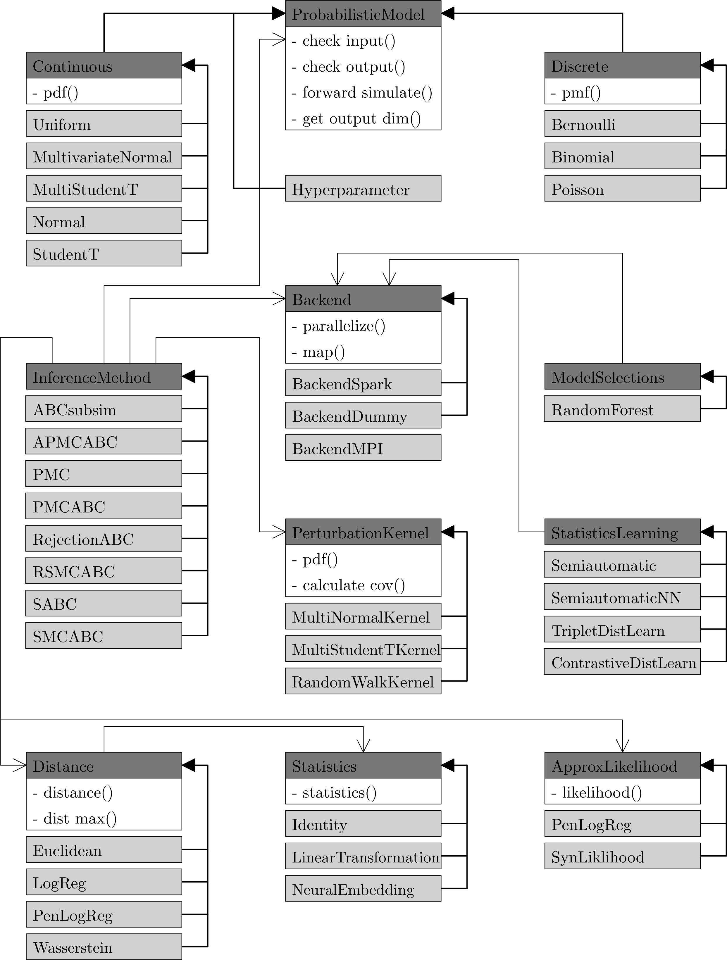
The following diagram shows selected classes with their most important
methods. Abstract classes, which cannot be instantiated, are highlighted in
dark gray and derived classes are highlighted in light gray. Inheritance is
shown by filled arrows. Arrows with no filling highlight associations, e.g.,
Distance is associated with Statistics
because it calls a method of the instantiated class to translate the input data to summary statistics.
abcpy.acceptedparametersmanager module
-
class
abcpy.acceptedparametersmanager.AcceptedParametersManager(model)[source]¶ Bases:
object-
__init__(model)[source]¶ This class manages the accepted parameters and other bds objects.
Parameters: model (list) – List of all root probabilistic models
-
broadcast(backend, observations)[source]¶ Broadcasts the observations to observations_bds using the specified backend.
Parameters: - backend (abcpy.backends object) – The backend used by the inference algorithm
- observations (list) – A list containing all observed data
-
update_kernel_values(backend, kernel_parameters)[source]¶ Broadcasts new parameters for each kernel
Parameters: - backend (abcpy.backends object) – The backend used by the inference algorithm
- kernel_parameters (list) – A list, in which each entry contains the values of the parameters associated with the corresponding kernel in the joint perturbation kernel
-
update_broadcast(backend, accepted_parameters=None, accepted_weights=None, accepted_cov_mats=None)[source]¶ Updates the broadcasted values using the specified backend
Parameters: - backend (abcpy.backend object) – The backend to be used for broadcasting
- accepted_parameters (list) – The accepted parameters to be broadcasted
- accepted_weights (list) – The accepted weights to be broadcasted
- accepted_cov_mats (np.ndarray) – The accepted covariance matrix to be broadcasted
-
get_mapping(models, is_root=True, index=0)[source]¶ Returns the order in which the models are discovered during recursive depth-first search. Commonly used when returning the accepted_parameters_bds for certain models.
Parameters: - models (list) – List of the root probabilistic models of the graph.
- is_root (boolean) – Specifies whether the current list of models is the list of overall root models
- index (integer) – The current index in depth-first search.
Returns: The first entry corresponds to the mapping of the root model, as well as all its parents. The second entry corresponds to the next index in depth-first search.
Return type: list
-
get_accepted_parameters_bds_values(models)[source]¶ Returns the accepted bds values for the specified models.
Parameters: models (list) – Contains the probabilistic models for which the accepted bds values should be returned Returns: The accepted_parameters_bds values of all the probabilistic models specified in models. Return type: list
-
abcpy.approx_lhd module
-
class
abcpy.approx_lhd.Approx_likelihood(statistics_calc)[source]¶ Bases:
objectThis abstract base class defines the approximate likelihood function.
-
__init__(statistics_calc)[source]¶ The constructor of a sub-class must accept a non-optional statistics calculator, which is stored to self.statistics_calc.
Parameters: statistics_calc (abcpy.stasistics.Statistics) – Statistics extractor object that conforms to the Statistics class.
-
loglikelihood(y_obs, y_sim)[source]¶ To be overwritten by any sub-class: should compute the approximate loglikelihood value given the observed data set y_obs and the data set y_sim simulated from model set at the parameter value.
Parameters: - y_obs (Python list) – Observed data set.
- y_sim (Python list) – Simulated data set from model at the parameter value.
Returns: Computed approximate loglikelihood.
Return type: float
-
-
class
abcpy.approx_lhd.SynLikelihood(statistics_calc)[source]¶ Bases:
abcpy.approx_lhd.Approx_likelihoodThis class implements the approximate likelihood function which computes the approximate likelihood using the synthetic likelihood approach described in Wood [1]. For synthetic likelihood approximation, we compute the robust precision matrix using Ledoit and Wolf’s [2] method.
[1] S. N. Wood. Statistical inference for noisy nonlinear ecological dynamic systems. Nature, 466(7310):1102–1104, Aug. 2010.
[2] O. Ledoit and M. Wolf, A Well-Conditioned Estimator for Large-Dimensional Covariance Matrices, Journal of Multivariate Analysis, Volume 88, Issue 2, pages 365-411, February 2004.
-
__init__(statistics_calc)[source]¶ The constructor of a sub-class must accept a non-optional statistics calculator, which is stored to self.statistics_calc.
Parameters: statistics_calc (abcpy.stasistics.Statistics) – Statistics extractor object that conforms to the Statistics class.
-
loglikelihood(y_obs, y_sim)[source]¶ To be overwritten by any sub-class: should compute the approximate loglikelihood value given the observed data set y_obs and the data set y_sim simulated from model set at the parameter value.
Parameters: - y_obs (Python list) – Observed data set.
- y_sim (Python list) – Simulated data set from model at the parameter value.
Returns: Computed approximate loglikelihood.
Return type: float
-
-
class
abcpy.approx_lhd.PenLogReg(statistics_calc, model, n_simulate, n_folds=10, max_iter=100000, seed=None)[source]¶ Bases:
abcpy.approx_lhd.Approx_likelihood,abcpy.graphtools.GraphToolsThis class implements the approximate likelihood function which computes the approximate likelihood up to a constant using penalized logistic regression described in Dutta et. al. [1]. It takes one additional function handler defining the true model and two additional parameters n_folds and n_simulate correspondingly defining number of folds used to estimate prediction error using cross-validation and the number of simulated dataset sampled from each parameter to approximate the likelihood function. For lasso penalized logistic regression we use glmnet of Friedman et. al. [2].
[1] Thomas, O., Dutta, R., Corander, J., Kaski, S., & Gutmann, M. U. (2020). Likelihood-free inference by ratio estimation. Bayesian Analysis.
[2] Friedman, J., Hastie, T., and Tibshirani, R. (2010). Regularization paths for generalized linear models via coordinate descent. Journal of Statistical Software, 33(1), 1–22.
Parameters: - statistics_calc (abcpy.statistics.Statistics) – Statistics extractor object that conforms to the Statistics class.
- model (abcpy.models.Model) – Model object that conforms to the Model class.
- n_simulate (int) – Number of data points to simulate for the reference data set; this has to be the same as n_samples_per_param when calling the sampler. The reference data set is generated by drawing parameters from the prior and samples from the model when PenLogReg is instantiated.
- n_folds (int, optional) – Number of folds for cross-validation. The default value is 10.
- max_iter (int, optional) – Maximum passes over the data. The default is 100000.
- seed (int, optional) – Seed for the random number generator. The used glmnet solver is not deterministic, this seed is used for determining the cv folds. The default value is None.
-
__init__(statistics_calc, model, n_simulate, n_folds=10, max_iter=100000, seed=None)[source]¶ The constructor of a sub-class must accept a non-optional statistics calculator, which is stored to self.statistics_calc.
Parameters: statistics_calc (abcpy.stasistics.Statistics) – Statistics extractor object that conforms to the Statistics class.
-
loglikelihood(y_obs, y_sim)[source]¶ To be overwritten by any sub-class: should compute the approximate loglikelihood value given the observed data set y_obs and the data set y_sim simulated from model set at the parameter value.
Parameters: - y_obs (Python list) – Observed data set.
- y_sim (Python list) – Simulated data set from model at the parameter value.
Returns: Computed approximate loglikelihood.
Return type: float
abcpy.backends module
-
class
abcpy.backends.base.Backend[source]¶ Bases:
objectThis is the base class for every parallelization backend. It essentially resembles the map/reduce API from Spark.
An idea for the future is to implement a MPI version of the backend with the hope to be more complient with standard HPC infrastructure and a potential speed-up.
-
parallelize(list)[source]¶ This method distributes the list on the available workers and returns a reference object.
The list should be split into number of workers many parts. Each part should then be sent to a separate worker node.
Parameters: list (Python list) – the list that should get distributed on the worker nodes Returns: A reference object that represents the parallelized list Return type: PDS class (parallel data set)
-
broadcast(object)[source]¶ Send object to all worker nodes without splitting it up.
Parameters: object (Python object) – An abitrary object that should be available on all workers Returns: A reference to the broadcasted object Return type: BDS class (broadcast data set)
-
map(func, pds)[source]¶ A distributed implementation of map that works on parallel data sets (PDS).
On every element of pds the function func is called.
Parameters: - func (Python func) – A function that can be applied to every element of the pds
- pds (PDS class) – A parallel data set to which func should be applied
Returns: a new parallel data set that contains the result of the map
Return type: PDS class
-
-
class
abcpy.backends.base.PDS[source]¶ Bases:
objectThe reference class for parallel data sets (PDS).
-
class
abcpy.backends.base.BDS[source]¶ Bases:
objectThe reference class for broadcast data set (BDS).
-
class
abcpy.backends.base.BackendDummy[source]¶ Bases:
abcpy.backends.base.BackendThis is a dummy parallelization backend, meaning it doesn’t parallelize anything. It is mainly implemented for testing purpose.
-
parallelize(python_list)[source]¶ This actually does nothing: it just wraps the Python list into dummy pds (PDSDummy).
Parameters: python_list (Python list) – Returns: Return type: PDSDummy (parallel data set)
-
broadcast(object)[source]¶ This actually does nothing: it just wraps the object into BDSDummy.
Parameters: object (Python object) – Returns: Return type: BDSDummy class
-
map(func, pds)[source]¶ This is a wrapper for the Python internal map function.
Parameters: - func (Python func) – A function that can be applied to every element of the pds
- pds (PDSDummy class) – A pseudo-parallel data set to which func should be applied
Returns: a new pseudo-parallel data set that contains the result of the map
Return type: PDSDummy class
-
-
class
abcpy.backends.base.PDSDummy(python_list)[source]¶ Bases:
abcpy.backends.base.PDSThis is a wrapper for a Python list to fake parallelization.
-
class
abcpy.backends.base.BDSDummy(object)[source]¶ Bases:
abcpy.backends.base.BDSThis is a wrapper for a Python object to fake parallelization.
-
class
abcpy.backends.spark.BackendSpark(sparkContext, parallelism=4)[source]¶ Bases:
abcpy.backends.base.BackendA parallelization backend for Apache Spark. It is essetially a wrapper for the required Spark functionality.
-
__init__(sparkContext, parallelism=4)[source]¶ Initialize the backend with an existing and configured SparkContext.
Parameters: - sparkContext (pyspark.SparkContext) – an existing and fully configured PySpark context
- parallelism (int) – defines on how many workers a distributed dataset can be distributed
-
parallelize(python_list)[source]¶ This is a wrapper of pyspark.SparkContext.parallelize().
Parameters: list (Python list) – list that is distributed on the workers Returns: A reference object that represents the parallelized list Return type: PDSSpark class (parallel data set)
-
broadcast(object)[source]¶ This is a wrapper for pyspark.SparkContext.broadcast().
Parameters: object (Python object) – An abitrary object that should be available on all workers Returns: A reference to the broadcasted object Return type: BDSSpark class (broadcast data set)
-
map(func, pds)[source]¶ This is a wrapper for pyspark.rdd.map()
Parameters: - func (Python func) – A function that can be applied to every element of the pds
- pds (PDSSpark class) – A parallel data set to which func should be applied
Returns: a new parallel data set that contains the result of the map
Return type: PDSSpark class
-
-
class
abcpy.backends.spark.PDSSpark(rdd)[source]¶ Bases:
abcpy.backends.base.PDSThis is a wrapper for Apache Spark RDDs.
-
class
abcpy.backends.spark.BDSSpark(bcv)[source]¶ Bases:
abcpy.backends.base.BDSThis is a wrapper for Apache Spark Broadcast variables.
abcpy.continuousmodels module
-
class
abcpy.continuousmodels.Uniform(parameters, name='Uniform')[source]¶ Bases:
abcpy.probabilisticmodels.ProbabilisticModel,abcpy.probabilisticmodels.Continuous-
__init__(parameters, name='Uniform')[source]¶ This class implements a probabilistic model following an uniform distribution.
Parameters: - parameters (list) – Contains two lists. The first list specifies the probabilistic models and hyperparameters from which the lower bound of the uniform distribution derive. The second list specifies the probabilistic models and hyperparameters from which the upper bound derives.
- name (string, optional) – The name that should be given to the probabilistic model in the journal file.
-
forward_simulate(input_values, k, rng=<MagicMock name='mock.RandomState()' id='139658057894608'>, mpi_comm=None)[source]¶ Samples from a uniform distribution using the current values for each probabilistic model from which the model derives.
Parameters: - input_values (list) – List of input parameters, in the same order as specified in the InputConnector passed to the init function
- k (integer) – The number of samples that should be drawn.
- rng (Random number generator) – Defines the random number generator to be used. The default value uses a random seed to initialize the generator.
Returns: list – A list containing the sampled values as np-array.
Return type: [np.ndarray]
-
get_output_dimension()[source]¶ Provides the output dimension of the current model.
This function is in particular important if the current model is used as an input for other models. In such a case it is assumed that the output is always a vector of int or float. The length of the vector is the dimension that should be returned here.
Returns: The dimension of the output vector of a single forward simulation. Return type: int
-
pdf(input_values, x)[source]¶ Calculates the probability density function at point x. Commonly used to determine whether perturbed parameters are still valid according to the pdf.
Parameters: - input_values (list) – List of input parameters, in the same order as specified in the InputConnector passed to the init function
- x (list) – The point at which the pdf should be evaluated.
Returns: The evaluated pdf at point x.
Return type: Float
-
-
class
abcpy.continuousmodels.Normal(parameters, name='Normal')[source]¶ Bases:
abcpy.probabilisticmodels.ProbabilisticModel,abcpy.probabilisticmodels.Continuous-
__init__(parameters, name='Normal')[source]¶ This class implements a probabilistic model following a normal distribution with mean mu and variance sigma.
Parameters: - parameters (list) – Contains the probabilistic models and hyperparameters from which the model derives. The list has two entries: from the first entry mean of the distribution and from the second entry variance is derived. Note that the second value of the list is strictly greater than 0.
- name (string) – The name that should be given to the probabilistic model in the journal file.
-
forward_simulate(input_values, k, rng=<MagicMock name='mock.RandomState()' id='139658057921424'>, mpi_comm=None)[source]¶ Samples from a normal distribution using the current values for each probabilistic model from which the model derives.
Parameters: - input_values (list) – List of input parameters, in the same order as specified in the InputConnector passed to the init function
- k (integer) – The number of samples that should be drawn.
- rng (Random number generator) – Defines the random number generator to be used. The default value uses a random seed to initialize the generator.
Returns: list – A list containing the sampled values as np-array.
Return type: [np.ndarray]
-
get_output_dimension()[source]¶ Provides the output dimension of the current model.
This function is in particular important if the current model is used as an input for other models. In such a case it is assumed that the output is always a vector of int or float. The length of the vector is the dimension that should be returned here.
Returns: The dimension of the output vector of a single forward simulation. Return type: int
-
pdf(input_values, x)[source]¶ Calculates the probability density function at point x. Commonly used to determine whether perturbed parameters are still valid according to the pdf.
Parameters: - input_values (list) – List of input parameters of the from [mu, sigma]
- x (list) – The point at which the pdf should be evaluated.
Returns: The evaluated pdf at point x.
Return type: Float
-
-
class
abcpy.continuousmodels.StudentT(parameters, name='StudentT')[source]¶ Bases:
abcpy.probabilisticmodels.ProbabilisticModel,abcpy.probabilisticmodels.Continuous-
__init__(parameters, name='StudentT')[source]¶ This class implements a probabilistic model following the Student’s T-distribution.
Parameters: - parameters (list) – Contains the probabilistic models and hyperparameters from which the model derives. The list has two entries: from the first entry mean of the distribution and from the second entry degrees of freedom is derived. Note that the second value of the list is strictly greater than 0.
- name (string) – The name that should be given to the probabilistic model in the journal file.
-
forward_simulate(input_values, k, rng=<MagicMock name='mock.RandomState()' id='139658057948304'>, mpi_comm=None)[source]¶ Samples from a Student’s T-distribution using the current values for each probabilistic model from which the model derives.
Parameters: - input_values (list) – List of input parameters, in the same order as specified in the InputConnector passed to the init function
- k (integer) – The number of samples that should be drawn.
- rng (Random number generator) – Defines the random number generator to be used. The default value uses a random seed to initialize the generator.
Returns: list – A list containing the sampled values as np-array.
Return type: [np.ndarray]
-
get_output_dimension()[source]¶ Provides the output dimension of the current model.
This function is in particular important if the current model is used as an input for other models. In such a case it is assumed that the output is always a vector of int or float. The length of the vector is the dimension that should be returned here.
Returns: The dimension of the output vector of a single forward simulation. Return type: int
-
pdf(input_values, x)[source]¶ Calculates the probability density function at point x. Commonly used to determine whether perturbed parameters are still valid according to the pdf.
Parameters: - input_values (list) – List of input parameters
- x (list) – The point at which the pdf should be evaluated.
Returns: The evaluated pdf at point x.
Return type: Float
-
-
class
abcpy.continuousmodels.MultivariateNormal(parameters, name='Multivariate Normal')[source]¶ Bases:
abcpy.probabilisticmodels.ProbabilisticModel,abcpy.probabilisticmodels.Continuous-
__init__(parameters, name='Multivariate Normal')[source]¶ This class implements a probabilistic model following a multivariate normal distribution with mean and covariance matrix.
Parameters: - parameters (list of at length 2) – Contains the probabilistic models and hyperparameters from which the model derives. The first entry defines the mean, while the second entry defines the Covariance matrix. Note that if the mean is n dimensional, the covariance matrix is required to be of dimension nxn, symmetric and positive-definite.
- name (string) – The name that should be given to the probabilistic model in the journal file.
-
forward_simulate(input_values, k, rng=<MagicMock name='mock.RandomState()' id='139658057983632'>, mpi_comm=None)[source]¶ Samples from a multivariate normal distribution using the current values for each probabilistic model from which the model derives.
Parameters: - input_values (list) – List of input parameters, in the same order as specified in the InputConnector passed to the init function
- k (integer) – The number of samples that should be drawn.
- rng (Random number generator) – Defines the random number generator to be used. The default value uses a random seed to initialize the generator.
Returns: list – A list containing the sampled values as np-array.
Return type: [np.ndarray]
-
get_output_dimension()[source]¶ Provides the output dimension of the current model.
This function is in particular important if the current model is used as an input for other models. In such a case it is assumed that the output is always a vector of int or float. The length of the vector is the dimension that should be returned here.
Returns: The dimension of the output vector of a single forward simulation. Return type: int
-
pdf(input_values, x)[source]¶ Calculates the probability density function at point x. Commonly used to determine whether perturbed parameters are still valid according to the pdf.
Parameters: - input_values (list) – List of input parameters
- x (list) – The point at which the pdf should be evaluated.
Returns: The evaluated pdf at point x.
Return type: Float
-
-
class
abcpy.continuousmodels.MultiStudentT(parameters, name='MultiStudentT')[source]¶ Bases:
abcpy.probabilisticmodels.ProbabilisticModel,abcpy.probabilisticmodels.Continuous-
__init__(parameters, name='MultiStudentT')[source]¶ This class implements a probabilistic model following the multivariate Student-T distribution.
Parameters: - parameters (list) – All but the last two entries contain the probabilistic models and hyperparameters from which the model derives. The second to last entry contains the covariance matrix. If the mean is of dimension n, the covariance matrix is required to be nxn dimensional. The last entry contains the degrees of freedom.
- name (string) – The name that should be given to the probabilistic model in the journal file.
-
forward_simulate(input_values, k, rng=<MagicMock name='mock.RandomState()' id='139658060415056'>, mpi_comm=None)[source]¶ Samples from a multivariate Student’s T-distribution using the current values for each probabilistic model from which the model derives.
Parameters: - input_values (list) – List of input parameters, in the same order as specified in the InputConnector passed to the init function
- k (integer) – The number of samples that should be drawn.
- rng (Random number generator) – Defines the random number generator to be used. The default value uses a random seed to initialize the generator.
Returns: list – A list containing the sampled values as np-array.
Return type: [np.ndarray]
-
get_output_dimension()[source]¶ Provides the output dimension of the current model.
This function is in particular important if the current model is used as an input for other models. In such a case it is assumed that the output is always a vector of int or float. The length of the vector is the dimension that should be returned here.
Returns: The dimension of the output vector of a single forward simulation. Return type: int
-
pdf(input_values, x)[source]¶ Calculates the probability density function at point x. Commonly used to determine whether perturbed parameters are still valid according to the pdf.
Parameters: - input_values (list) – List of input parameters
- x (list) – The point at which the pdf should be evaluated.
Returns: The evaluated pdf at point x.
Return type: Float
-
abcpy.discretemodels module
-
class
abcpy.discretemodels.Bernoulli(parameters, name='Bernoulli')[source]¶ Bases:
abcpy.probabilisticmodels.Discrete,abcpy.probabilisticmodels.ProbabilisticModel-
__init__(parameters, name='Bernoulli')[source]¶ This class implements a probabilistic model following a bernoulli distribution.
Parameters: - parameters (list) – A list containing one entry, the probability of the distribution.
- name (string) – The name that should be given to the probabilistic model in the journal file.
-
forward_simulate(input_values, k, rng=<MagicMock name='mock.RandomState()' id='139658058699536'>, mpi_comm=None)[source]¶ Samples from the bernoulli distribution associtated with the probabilistic model.
Parameters: - input_values (list) – List of input parameters, in the same order as specified in the InputConnector passed to the init function
- k (integer) – The number of samples to be drawn.
- rng (random number generator) – The random number generator to be used.
Returns: list – A list containing the sampled values as np-array.
Return type: [np.ndarray]
-
get_output_dimension()[source]¶ Provides the output dimension of the current model.
This function is in particular important if the current model is used as an input for other models. In such a case it is assumed that the output is always a vector of int or float. The length of the vector is the dimension that should be returned here.
Returns: The dimension of the output vector of a single forward simulation. Return type: int
-
pmf(input_values, x)[source]¶ Evaluates the probability mass function at point x.
Parameters: - input_values (list) – List of input parameters, in the same order as specified in the InputConnector passed to the init function
- x (float) – The point at which the pmf should be evaluated.
Returns: The pmf evaluated at point x.
Return type: float
-
-
class
abcpy.discretemodels.Binomial(parameters, name='Binomial')[source]¶ Bases:
abcpy.probabilisticmodels.Discrete,abcpy.probabilisticmodels.ProbabilisticModel-
__init__(parameters, name='Binomial')[source]¶ This class implements a probabilistic model following a binomial distribution.
Parameters: - parameters (list) – Contains the probabilistic models and hyperparameters from which the model derives. Note that the first entry of the list, n, an integer and has to be larger than or equal to 0, while the second entry, p, has to be in the interval [0,1].
- name (string) – The name that should be given to the probabilistic model in the journal file.
-
forward_simulate(input_values, k, rng=<MagicMock name='mock.RandomState()' id='139658057438544'>, mpi_comm=None)[source]¶ Samples from a binomial distribution using the current values for each probabilistic model from which the model derives.
Parameters: - input_values (list) – List of input parameters, in the same order as specified in the InputConnector passed to the init function
- k (integer) – The number of samples that should be drawn.
- rng (Random number generator) – Defines the random number generator to be used. The default value uses a random seed to initialize the generator.
Returns: list – A list containing the sampled values as np-array.
Return type: [np.ndarray]
-
get_output_dimension()[source]¶ Provides the output dimension of the current model.
This function is in particular important if the current model is used as an input for other models. In such a case it is assumed that the output is always a vector of int or float. The length of the vector is the dimension that should be returned here.
Returns: The dimension of the output vector of a single forward simulation. Return type: int
-
pmf(input_values, x)[source]¶ Calculates the probability mass function at point x.
Parameters: - input_values (list) – List of input parameters, in the same order as specified in the InputConnector passed to the init function
- x (list) – The point at which the pmf should be evaluated.
Returns: The evaluated pmf at point x.
Return type: Float
-
-
class
abcpy.discretemodels.Poisson(parameters, name='Poisson')[source]¶ Bases:
abcpy.probabilisticmodels.Discrete,abcpy.probabilisticmodels.ProbabilisticModel-
__init__(parameters, name='Poisson')[source]¶ This class implements a probabilistic model following a poisson distribution.
Parameters: - parameters (list) – A list containing one entry, the mean of the distribution.
- name (string) – The name that should be given to the probabilistic model in the journal file.
-
forward_simulate(input_values, k, rng=<MagicMock name='mock.RandomState()' id='139658057179536'>, mpi_comm=None)[source]¶ Samples k values from the defined possion distribution.
Parameters: - input_values (list) – List of input parameters, in the same order as specified in the InputConnector passed to the init function
- k (integer) – The number of samples.
- rng (random number generator) – The random number generator to be used.
Returns: list – A list containing the sampled values as np-array.
Return type: [np.ndarray]
-
get_output_dimension()[source]¶ Provides the output dimension of the current model.
This function is in particular important if the current model is used as an input for other models. In such a case it is assumed that the output is always a vector of int or float. The length of the vector is the dimension that should be returned here.
Returns: The dimension of the output vector of a single forward simulation. Return type: int
-
pmf(input_values, x)[source]¶ Calculates the probability mass function of the distribution at point x.
Parameters: - input_values (list) – List of input parameters, in the same order as specified in the InputConnector passed to the init function
- x (integer) – The point at which the pmf should be evaluated.
Returns: The evaluated pmf at point x.
Return type: Float
-
-
class
abcpy.discretemodels.DiscreteUniform(parameters, name='DiscreteUniform')[source]¶ Bases:
abcpy.probabilisticmodels.Discrete,abcpy.probabilisticmodels.ProbabilisticModel-
__init__(parameters, name='DiscreteUniform')[source]¶ This class implements a probabilistic model following a Discrete Uniform distribution.
Parameters: - parameters (list) – A list containing two entries, the upper and lower bound of the range.
- name (string) – The name that should be given to the probabilistic model in the journal file.
-
forward_simulate(input_values, k, rng=<MagicMock name='mock.RandomState()' id='139658057173008'>)[source]¶ Samples from the Discrete Uniform distribution associated with the probabilistic model.
Parameters: - input_values (list) – List of input parameters, in the same order as specified in the InputConnector passed to the init function
- k (integer) – The number of samples to be drawn.
- rng (random number generator) – The random number generator to be used.
Returns: list – A list containing the sampled values as np-array.
Return type: [np.ndarray]
-
get_output_dimension()[source]¶ Provides the output dimension of the current model.
This function is in particular important if the current model is used as an input for other models. In such a case it is assumed that the output is always a vector of int or float. The length of the vector is the dimension that should be returned here.
Returns: The dimension of the output vector of a single forward simulation. Return type: int
-
pmf(input_values, x)[source]¶ Evaluates the probability mass function at point x.
Parameters: - input_values (list) – List of input parameters, in the same order as specified in the InputConnector passed to the init function
- x (float) – The point at which the pmf should be evaluated.
Returns: The pmf evaluated at point x.
Return type: float
-
abcpy.distances module
-
class
abcpy.distances.Distance(statistics_calc)[source]¶ Bases:
objectThis abstract base class defines how the distance between the observed and simulated data should be implemented.
-
__init__(statistics_calc)[source]¶ The constructor of a sub-class must accept a non-optional statistics calculator as a parameter; then, it must call the __init__ method of the parent class. This ensures that the object is initialized correctly so that the _calculate_summary_stat private method can be called when computing the distances.
Parameters: statistics_calc (abcpy.statistics.Statistics) – Statistics extractor object that conforms to the Statistics class.
-
distance(d1, d2)[source]¶ To be overwritten by any sub-class: should calculate the distance between two sets of data d1 and d2 using their respective statistics.
Usually, calling the _calculate_summary_stat private method to obtain statistics from the datasets is handy; that also keeps track of the first provided dataset (which is the observation in ABCpy inference schemes) and avoids computing the statistics for that multiple times.
Notes
The data sets d1 and d2 are array-like structures that contain n1 and n2 data points each. An implementation of the distance function should work along the following steps:
1. Transform both input sets dX = [ dX1, dX2, …, dXn ] to sX = [sX1, sX2, …, sXn] using the statistics object. See _calculate_summary_stat method.
2. Calculate the mutual desired distance, here denoted by - between the statistics; for instance, dist = [s11 - s21, s12 - s22, …, s1n - s2n] (in some cases however you may want to compute all pairwise distances between statistics elements.
Important: any sub-class must not calculate the distance between data sets d1 and d2 directly. This is the reason why any sub-class must be initialized with a statistics object.
Parameters: - d1 (Python list) – Contains n1 data points.
- d2 (Python list) – Contains n2 data points.
Returns: The distance between the two input data sets.
Return type: numpy.float
-
dist_max()[source]¶ To be overwritten by sub-class: should return maximum possible value of the desired distance function.
Examples
If the desired distance maps to \(\mathbb{R}\), this method should return numpy.inf.
Returns: The maximal possible value of the desired distance function. Return type: numpy.float
-
-
class
abcpy.distances.Euclidean(statistics)[source]¶ Bases:
abcpy.distances.DistanceThis class implements the Euclidean distance between two vectors.
The maximum value of the distance is np.inf.
-
__init__(statistics)[source]¶ Parameters: statistics_calc (abcpy.statistics.Statistics) – Statistics extractor object that conforms to the Statistics class.
-
distance(d1, d2)[source]¶ Calculates the distance between two datasets, by computing Euclidean distance between each element of d1 and d2 and taking their average.
Parameters: - d1 (Python list) – Contains n1 data points.
- d2 (Python list) – Contains n2 data points.
Returns: The distance between the two input data sets.
Return type: numpy.float
-
-
class
abcpy.distances.PenLogReg(statistics)[source]¶ Bases:
abcpy.distances.DistanceThis class implements a distance measure based on the classification accuracy.
The classification accuracy is calculated between two dataset d1 and d2 using lasso penalized logistics regression and return it as a distance. The lasso penalized logistic regression is done using glmnet package of Friedman et. al. [2]. While computing the distance, the algorithm automatically chooses the most relevant summary statistics as explained in Gutmann et. al. [1]. The maximum value of the distance is 1.0.
[1] Gutmann, M. U., Dutta, R., Kaski, S., & Corander, J. (2018). Likelihood-free inference via classification. Statistics and Computing, 28(2), 411-425.
[2] Friedman, J., Hastie, T., and Tibshirani, R. (2010). Regularization paths for generalized linear models via coordinate descent. Journal of Statistical Software, 33(1), 1–22.
-
__init__(statistics)[source]¶ Parameters: statistics_calc (abcpy.statistics.Statistics) – Statistics extractor object that conforms to the Statistics class.
-
-
class
abcpy.distances.LogReg(statistics, seed=None)[source]¶ Bases:
abcpy.distances.DistanceThis class implements a distance measure based on the classification accuracy [1]. The classification accuracy is calculated between two dataset d1 and d2 using logistics regression and return it as a distance. The maximum value of the distance is 1.0. The logistic regression may not converge when using one single sample in each dataset (as for instance by putting n_samples_per_param=1 in an inference routine).
[1] Gutmann, M. U., Dutta, R., Kaski, S., & Corander, J. (2018). Likelihood-free inference via classification. Statistics and Computing, 28(2), 411-425.
-
__init__(statistics, seed=None)[source]¶ Parameters: - statistics_calc (abcpy.statistics.Statistics) – Statistics extractor object that conforms to the Statistics class.
- seed (integer, optionl) – Seed used to initialize the Random Numbers Generator used to determine the (random) cross validation split in the Logistic Regression classifier.
-
-
class
abcpy.distances.Wasserstein(statistics, num_iter_max=100000)[source]¶ Bases:
abcpy.distances.DistanceThis class implements a distance measure based on the 2-Wasserstein distance, as used in [1]. This considers the several simulations/observations in the datasets as iid samples from the model for a fixed parameter value/from the data generating model, and computes the 2-Wasserstein distance between the empirical distributions those simulations/observations define.
[1] Bernton, E., Jacob, P.E., Gerber, M. and Robert, C.P. (2019), Approximate Bayesian computation with the Wasserstein distance. J. R. Stat. Soc. B, 81: 235-269. doi:10.1111/rssb.12312
-
__init__(statistics, num_iter_max=100000)[source]¶ Parameters: - statistics_calc (abcpy.statistics.Statistics) – Statistics extractor object that conforms to the Statistics class.
- num_iter_max (integer, optional) – The maximum number of iterations in the linear programming algorithm to estimate the Wasserstein distance. Default to 100000.
-
abcpy.graphtools module
-
class
abcpy.graphtools.GraphTools[source]¶ Bases:
objectThis class implements all methods that will be called recursively on the graph structure.
-
sample_from_prior(model=None, rng=<MagicMock name='mock.RandomState()' id='139658061730000'>)[source]¶ Samples values for all random variables of the model. Commonly used to sample new parameter values on the whole graph.
Parameters: - model (abcpy.ProbabilisticModel object) – The root model for which sample_from_prior should be called.
- rng (Random number generator) – Defines the random number generator to be used
-
pdf_of_prior(models, parameters, mapping=None, is_root=True)[source]¶ Calculates the joint probability density function of the prior of the specified models at the given parameter values. Commonly used to check whether new parameters are valid given the prior, as well as to calculate acceptance probabilities.
Parameters: - models (list of abcpy.ProbabilisticModel objects) – Defines the models for which the pdf of their prior should be evaluated
- parameters (python list) – The parameters at which the pdf should be evaluated
- mapping (list of tuples) – Defines the mapping of probabilistic models and index in a parameter list.
- is_root (boolean) – A flag specifying whether the provided models are the root models. This is to ensure that the pdf is calculated correctly.
Returns: The resulting pdf,as well as the next index to be considered in the parameters list.
Return type: list
-
get_parameters(models=None, is_root=True)[source]¶ Returns the current values of all free parameters in the model. Commonly used before perturbing the parameters of the model.
Parameters: - models (list of abcpy.ProbabilisticModel objects) – The models for which, together with their parents, the parameter values should be returned. If no value is provided, the root models are assumed to be the model of the inference method.
- is_root (boolean) – Specifies whether the current models are at the root. This ensures that the values corresponding to simulated observations will not be returned.
Returns: A list containing all currently sampled values of the free parameters.
Return type: list
-
set_parameters(parameters, models=None, index=0, is_root=True)[source]¶ Sets new values for the currently used values of each random variable. Commonly used after perturbing the parameter values using a kernel.
Parameters: - parameters (list) – Defines the values to which the respective parameter values of the models should be set
- model (list of abcpy.ProbabilisticModel objects) – Defines all models for which, together with their parents, new values should be set. If no value is provided, the root models are assumed to be the model of the inference method.
- index (integer) – The current index to be considered in the parameters list
- is_root (boolean) – Defines whether the current models are at the root. This ensures that only values corresponding to random variables will be set.
Returns: list – Returns whether it was possible to set all parameters and the next index to be considered in the parameters list.
Return type: [boolean, integer]
-
get_correct_ordering(parameters_and_models, models=None, is_root=True)[source]¶ Orders the parameters returned by a kernel in the order required by the graph. Commonly used when perturbing the parameters.
Parameters: - parameters_and_models (list of tuples) – Contains tuples containing as the first entry the probabilistic model to be considered and as the second entry the parameter values associated with this model
- models (list) – Contains the root probabilistic models that make up the graph. If no value is provided, the root models are assumed to be the model of the inference method.
Returns: The ordering which can be used by recursive functions on the graph.
Return type: list
-
simulate(n_samples_per_param, rng=<MagicMock name='mock.RandomState()' id='139658060195472'>, npc=None)[source]¶ Simulates data of each model using the currently sampled or perturbed parameters.
Parameters: rng (random number generator) – The random number generator to be used. Returns: Each entry corresponds to the simulated data of one model. Return type: list
-
abcpy.inferences module
-
class
abcpy.inferences.InferenceMethod[source]¶ Bases:
abcpy.graphtools.GraphToolsThis abstract base class represents an inference method.
-
sample()[source]¶ To be overwritten by any sub-class: Samples from the posterior distribution of the model parameter given the observed data observations.
-
model¶ an attribute specifying the model to be used
Type: To be overwritten by any sub-class
-
rng¶ an attribute specifying the random number generator to be used
Type: To be overwritten by any sub-class
-
backend¶ an attribute specifying the backend to be used.
Type: To be overwritten by any sub-class
-
n_samples¶ an attribute specifying the number of samples to be generated
Type: To be overwritten by any sub-class
-
n_samples_per_param¶ an attribute specifying the number of data points in each simulated data set.
Type: To be overwritten by any sub-class
-
-
class
abcpy.inferences.BaseMethodsWithKernel[source]¶ Bases:
objectThis abstract base class represents inference methods that have a kernel.
-
kernel¶ an attribute specifying the transition or perturbation kernel.
Type: To be overwritten by any sub-class
-
perturb(column_index, epochs=10, rng=<MagicMock name='mock.RandomState()' id='139658055972944'>)[source]¶ Perturbs all free parameters, given the current weights. Commonly used during inference.
Parameters: - column_index (integer) – The index of the column in the accepted_parameters_bds that should be used for perturbation
- epochs (integer) – The number of times perturbation should happen before the algorithm is terminated
Returns: Whether it was possible to set new parameter values for all probabilistic models
Return type: boolean
-
-
class
abcpy.inferences.BaseLikelihood[source]¶ Bases:
abcpy.inferences.InferenceMethod,abcpy.inferences.BaseMethodsWithKernelThis abstract base class represents inference methods that use the likelihood.
-
likfun¶ an attribute specifying the likelihood function to be used.
Type: To be overwritten by any sub-class
-
-
class
abcpy.inferences.BaseDiscrepancy[source]¶ Bases:
abcpy.inferences.InferenceMethod,abcpy.inferences.BaseMethodsWithKernelThis abstract base class represents inference methods using descrepancy.
-
distance¶ an attribute specifying the distance function.
Type: To be overwritten by any sub-class
-
-
class
abcpy.inferences.RejectionABC(root_models, distances, backend, seed=None)[source]¶ Bases:
abcpy.inferences.InferenceMethodThis class implements the rejection algorithm based inference scheme [1] for Approximate Bayesian Computation.
[1] Tavaré, S., Balding, D., Griffith, R., Donnelly, P.: Inferring coalescence times from DNA sequence data. Genetics 145(2), 505–518 (1997).
Parameters: - model (list) – A list of the Probabilistic models corresponding to the observed datasets
- distance (abcpy.distances.Distance) – Distance object defining the distance measure to compare simulated and observed data sets.
- backend (abcpy.backends.Backend) – Backend object defining the backend to be used.
- seed (integer, optionaldistance) – Optional initial seed for the random number generator. The default value is generated randomly.
-
n_samples= None
-
n_samples_per_param= None
-
epsilon= None
-
__init__(root_models, distances, backend, seed=None)[source]¶ Initialize self. See help(type(self)) for accurate signature.
-
model= None
-
distance= None
-
backend= None
-
rng= None
-
sample(observations, n_samples, n_samples_per_param, epsilon, full_output=0)[source]¶ Samples from the posterior distribution of the model parameter given the observed data observations.
Parameters: - observations (list) – A list, containing lists describing the observed data sets
- n_samples (integer) – Number of samples to generate
- n_samples_per_param (integer) – Number of data points in each simulated data set.
- epsilon (float) – Value of threshold
- full_output (integer, optional) – If full_output==1, intermediate results are included in output journal. The default value is 0, meaning the intermediate results are not saved.
Returns: a journal containing simulation results, metadata and optionally intermediate results.
Return type:
-
class
abcpy.inferences.PMCABC(root_models, distances, backend, kernel=None, seed=None)[source]¶ Bases:
abcpy.inferences.BaseDiscrepancy,abcpy.inferences.InferenceMethodThis class implements a modified version of Population Monte Carlo based inference scheme for Approximate Bayesian computation of Beaumont et. al. [1]. Here the threshold value at t-th generation are adaptively chosen by taking the maximum between the epsilon_percentile-th value of discrepancies of the accepted parameters at t-1-th generation and the threshold value provided for this generation by the user. If we take the value of epsilon_percentile to be zero (default), this method becomes the inference scheme described in [1], where the threshold values considered at each generation are the ones provided by the user.
[1] M. A. Beaumont. Approximate Bayesian computation in evolution and ecology. Annual Review of Ecology, Evolution, and Systematics, 41(1):379–406, Nov. 2010.
Parameters: - model (list) – A list of the Probabilistic models corresponding to the observed datasets
- distance (abcpy.distances.Distance) – Distance object defining the distance measure to compare simulated and observed data sets.
- kernel (abcpy.distributions.Distribution) – Distribution object defining the perturbation kernel needed for the sampling.
- backend (abcpy.backends.Backend) – Backend object defining the backend to be used.
- seed (integer, optional) – Optional initial seed for the random number generator. The default value is generated randomly.
-
n_samples= 2
-
n_samples_per_param= None
-
__init__(root_models, distances, backend, kernel=None, seed=None)[source]¶ Initialize self. See help(type(self)) for accurate signature.
-
model= None
-
distance= None
-
kernel= None
-
backend= None
-
rng= None
-
sample(observations, steps, epsilon_init, n_samples=10000, n_samples_per_param=1, epsilon_percentile=10, covFactor=2, full_output=0, journal_file=None)[source]¶ Samples from the posterior distribution of the model parameter given the observed data observations.
Parameters: - observations (list) – A list, containing lists describing the observed data sets
- steps (integer) – Number of iterations in the sequential algoritm (“generations”)
- epsilon_init (numpy.ndarray) – An array of proposed values of epsilon to be used at each steps. Can be supplied A single value to be used as the threshold in Step 1 or a steps-dimensional array of values to be used as the threshold in evry steps.
- n_samples (integer, optional) – Number of samples to generate. The default value is 10000.
- n_samples_per_param (integer, optional) – Number of data points in each simulated data set. The default value is 1.
- epsilon_percentile (float, optional) – A value between [0, 100]. The default value is 10.
- covFactor (float, optional) – scaling parameter of the covariance matrix. The default value is 2 as considered in [1].
- full_output (integer, optional) – If full_output==1, intermediate results are included in output journal. The default value is 0, meaning the intermediate results are not saved.
- journal_file (str, optional) – Filename of a journal file to read an already saved journal file, from which the first iteration will start. The default value is None.
Returns: A journal containing simulation results, metadata and optionally intermediate results.
Return type:
-
class
abcpy.inferences.PMC(root_models, loglikfuns, backend, kernel=None, seed=None)[source]¶ Bases:
abcpy.inferences.BaseLikelihood,abcpy.inferences.InferenceMethodPopulation Monte Carlo based inference scheme of Cappé et. al. [1].
This algorithm assumes a likelihood function is available and can be evaluated at any parameter value given the oberved dataset. In absence of the likelihood function or when it can’t be evaluated with a rational computational expenses, we use the approximated likelihood functions in abcpy.approx_lhd module, for which the argument of the consistency of the inference schemes are based on Andrieu and Roberts [2].
[1] Cappé, O., Guillin, A., Marin, J.-M., and Robert, C. P. (2004). Population Monte Carlo. Journal of Computational and Graphical Statistics, 13(4), 907–929.
[2] C. Andrieu and G. O. Roberts. The pseudo-marginal approach for efficient Monte Carlo computations. Annals of Statistics, 37(2):697–725, 04 2009.
Parameters: - model (list) – A list of the Probabilistic models corresponding to the observed datasets
- loglikfun (abcpy.approx_lhd.Approx_likelihood) – Approx_loglikelihood object defining the approximated loglikelihood to be used.
- kernel (abcpy.distributions.Distribution) – Distribution object defining the perturbation kernel needed for the sampling.
- backend (abcpy.backends.Backend) – Backend object defining the backend to be used.
- seed (integer, optional) – Optional initial seed for the random number generator. The default value is generated randomly.
-
n_samples= None
-
n_samples_per_param= None
-
__init__(root_models, loglikfuns, backend, kernel=None, seed=None)[source]¶ Initialize self. See help(type(self)) for accurate signature.
-
model= None
-
likfun= None
-
kernel= None
-
backend= None
-
rng= None
-
sample(observations, steps, n_samples=10000, n_samples_per_param=100, covFactors=None, iniPoints=None, full_output=0, journal_file=None)[source]¶ Samples from the posterior distribution of the model parameter given the observed data observations.
Parameters: - observations (list) – A list, containing lists describing the observed data sets
- steps (integer) – number of iterations in the sequential algoritm (“generations”)
- n_samples (integer, optional) – number of samples to generate. The default value is 10000.
- n_samples_per_param (integer, optional) – number of data points in each simulated data set. The default value is 100.
- covFactors (list of float, optional) – scaling parameter of the covariance matrix. The default is a p dimensional array of 1 when p is the dimension of the parameter.
- inipoints (numpy.ndarray, optional) – parameter vaulues from where the sampling starts. By default sampled from the prior.
- full_output (integer, optional) – If full_output==1, intermediate results are included in output journal. The default value is 0, meaning the intermediate results are not saved.
- journal_file (str, optional) – Filename of a journal file to read an already saved journal file, from which the first iteration will start. The default value is None.
Returns: A journal containing simulation results, metadata and optionally intermediate results.
Return type:
-
class
abcpy.inferences.SABC(root_models, distances, backend, kernel=None, seed=None)[source]¶ Bases:
abcpy.inferences.BaseDiscrepancy,abcpy.inferences.InferenceMethodThis class implements a modified version of Simulated Annealing Approximate Bayesian Computation (SABC) of [1] when the prior is non-informative.
[1] C. Albert, H. R. Kuensch and A. Scheidegger. A Simulated Annealing Approach to Approximate Bayes Computations. Statistics and Computing, (2014).
Parameters: - model (list) – A list of the Probabilistic models corresponding to the observed datasets
- distance (abcpy.distances.Distance) – Distance object defining the distance measure used to compare simulated and observed data sets.
- kernel (abcpy.distributions.Distribution) – Distribution object defining the perturbation kernel needed for the sampling.
- backend (abcpy.backends.Backend) – Backend object defining the backend to be used.
- seed (integer, optional) – Optional initial seed for the random number generator. The default value is generated randomly.
-
n_samples= None
-
n_samples_per_param= None
-
epsilon= None
-
__init__(root_models, distances, backend, kernel=None, seed=None)[source]¶ Initialize self. See help(type(self)) for accurate signature.
-
model= None
-
distance= None
-
kernel= None
-
backend= None
-
rng= None
-
smooth_distances_bds= None
-
all_distances_bds= None
-
sample(observations, steps, epsilon, n_samples=10000, n_samples_per_param=1, beta=2, delta=0.2, v=0.3, ar_cutoff=0.1, resample=None, n_update=None, full_output=0, journal_file=None)[source]¶ Samples from the posterior distribution of the model parameter given the observed data observations.
Parameters: - observations (list) – A list, containing lists describing the observed data sets
- steps (integer) – Number of maximum iterations in the sequential algoritm (“generations”)
- epsilon (numpy.float) – A proposed value of threshold to start with.
- n_samples (integer, optional) – Number of samples to generate. The default value is 10000.
- n_samples_per_param (integer, optional) – Number of data points in each simulated data set. The default value is 1.
- beta (numpy.float, optional) – Tuning parameter of SABC, default value is 2. Used to scale up the covariance matrices obtained from data.
- delta (numpy.float, optional) – Tuning parameter of SABC, default value is 0.2.
- v (numpy.float, optional) – Tuning parameter of SABC, The default value is 0.3.
- ar_cutoff (numpy.float, optional) – Acceptance ratio cutoff: if the acceptance rate at some iteration of the algorithm is lower than that, the algorithm will stop. The default value is 0.1.
- resample (int, optional) – At any iteration, perform a resampling step if the number of accepted particles is larger than resample. When not provided, it assumes resample to be equal to n_samples.
- n_update (int, optional) – Number of perturbed parameters at each step, The default value is None which takes value inside n_samples
- full_output (integer, optional) – If full_output==1, intermediate results are included in output journal. The default value is 0, meaning the intermediate results are not saved.
- journal_file (str, optional) – Filename of a journal file to read an already saved journal file, from which the first iteration will start. The default value is None.
Returns: A journal containing simulation results, metadata and optionally intermediate results.
Return type:
-
class
abcpy.inferences.ABCsubsim(root_models, distances, backend, kernel=None, seed=None)[source]¶ Bases:
abcpy.inferences.BaseDiscrepancy,abcpy.inferences.InferenceMethodThis class implements Approximate Bayesian Computation by subset simulation (ABCsubsim) algorithm of [1].
[1] M. Chiachio, J. L. Beck, J. Chiachio, and G. Rus., Approximate Bayesian computation by subset simulation. SIAM J. Sci. Comput., 36(3):A1339–A1358, 2014/10/03 2014.
Parameters: - model (list) – A list of the Probabilistic models corresponding to the observed datasets
- distance (abcpy.distances.Distance) – Distance object defining the distance used to compare the simulated and observed data sets.
- kernel (abcpy.distributions.Distribution) – Distribution object defining the perturbation kernel needed for the sampling.
- backend (abcpy.backends.Backend) – Backend object defining the backend to be used.
- seed (integer, optional) – Optional initial seed for the random number generator. The default value is generated randomly.
-
n_samples= None
-
n_samples_per_param= None
-
chain_length= None
-
__init__(root_models, distances, backend, kernel=None, seed=None)[source]¶ Initialize self. See help(type(self)) for accurate signature.
-
model= None
-
distance= None
-
kernel= None
-
backend= None
-
rng= None
-
anneal_parameter= None
-
sample(observations, steps, n_samples=10000, n_samples_per_param=1, chain_length=10, ap_change_cutoff=10, full_output=0, journal_file=None)[source]¶ Samples from the posterior distribution of the model parameter given the observed data observations.
Parameters: - observations (list) – A list, containing lists describing the observed data sets
- steps (integer) – Number of iterations in the sequential algoritm (“generations”)
- n_samples (integer, optional) – Number of samples to generate. The default value is 10000.
- n_samples_per_param (integer, optional) – Number of data points in each simulated data set. The default value is 1.
- chain_length (int, optional) – The length of chains, default value is 10. But should be checked such that this is an divisor of n_samples.
- ap_change_cutoff (float, optional) – The cutoff value for the percentage change in the anneal parameter. If the change is less than ap_change_cutoff the iterations are stopped. The default value is 10.
- full_output (integer, optional) – If full_output==1, intermediate results are included in output journal. The default value is 0, meaning the intermediate results are not saved.
- journal_file (str, optional) – Filename of a journal file to read an already saved journal file, from which the first iteration will start. The default value is None.
Returns: A journal containing simulation results, metadata and optionally intermediate results.
Return type:
-
class
abcpy.inferences.RSMCABC(root_models, distances, backend, kernel=None, seed=None)[source]¶ Bases:
abcpy.inferences.BaseDiscrepancy,abcpy.inferences.InferenceMethodThis class implements Replenishment Sequential Monte Carlo Approximate Bayesian computation of Drovandi and Pettitt [1].
[1] CC. Drovandi CC and AN. Pettitt, Estimation of parameters for macroparasite population evolution using approximate Bayesian computation. Biometrics 67(1):225–233, 2011.
Parameters: - model (list) – A list of the Probabilistic models corresponding to the observed datasets
- distance (abcpy.distances.Distance) – Distance object defining the distance measure used to compare simulated and observed data sets.
- kernel (abcpy.distributions.Distribution) – Distribution object defining the perturbation kernel needed for the sampling.
- backend (abcpy.backends.Backend) – Backend object defining the backend to be used.
- seed (integer, optional) – Optional initial seed for the random number generator. The default value is generated randomly.
-
n_samples= None
-
n_samples_per_param= None
-
alpha= None
-
__init__(root_models, distances, backend, kernel=None, seed=None)[source]¶ Initialize self. See help(type(self)) for accurate signature.
-
model= None
-
distance= None
-
kernel= None
-
backend= None
-
R= None
-
rng= None
-
accepted_dist_bds= None
-
sample(observations, steps, n_samples=10000, n_samples_per_param=1, alpha=0.1, epsilon_init=100, epsilon_final=0.1, const=0.01, covFactor=2.0, full_output=0, journal_file=None)[source]¶ Samples from the posterior distribution of the model parameter given the observed data observations.
Parameters: - observations (list) – A list, containing lists describing the observed data sets
- steps (integer) – Number of iterations in the sequential algoritm (“generations”)
- n_samples (integer, optional) – Number of samples to generate. The default value is 10000.
- n_samples_per_param (integer, optional) – Number of data points in each simulated data set. The default value is 1.
- alpha (float, optional) – A parameter taking values between [0,1], the default value is 0.1.
- epsilon_init (float, optional) – Initial value of threshold, the default is 100
- epsilon_final (float, optional) – Terminal value of threshold, the default is 0.1
- const (float, optional) – A constant to compute acceptance probability, the default is 0.01.
- covFactor (float, optional) – scaling parameter of the covariance matrix. The default value is 2.
- full_output (integer, optional) – If full_output==1, intermediate results are included in output journal. The default value is 0, meaning the intermediate results are not saved.
- journal_file (str, optional) – Filename of a journal file to read an already saved journal file, from which the first iteration will start. The default value is None.
Returns: A journal containing simulation results, metadata and optionally intermediate results.
Return type:
-
class
abcpy.inferences.APMCABC(root_models, distances, backend, kernel=None, seed=None)[source]¶ Bases:
abcpy.inferences.BaseDiscrepancy,abcpy.inferences.InferenceMethodThis class implements Adaptive Population Monte Carlo Approximate Bayesian computation of M. Lenormand et al. [1].
[1] M. Lenormand, F. Jabot and G. Deffuant, Adaptive approximate Bayesian computation for complex models. Computational Statistics, 28:2777–2796, 2013.
Parameters: - model (list) – A list of the Probabilistic models corresponding to the observed datasets
- distance (abcpy.distances.Distance) – Distance object defining the distance measure used to compare simulated and observed data sets.
- kernel (abcpy.distributions.Distribution) – Distribution object defining the perturbation kernel needed for the sampling.
- backend (abcpy.backends.Backend) – Backend object defining the backend to be used.
- seed (integer, optional) – Optional initial seed for the random number generator. The default value is generated randomly.
-
n_samples= None
-
n_samples_per_param= None
-
alpha= None
-
accepted_dist= None
-
__init__(root_models, distances, backend, kernel=None, seed=None)[source]¶ Initialize self. See help(type(self)) for accurate signature.
-
model= None
-
distance= None
-
kernel= None
-
backend= None
-
epsilon= None
-
rng= None
-
sample(observations, steps, n_samples=10000, n_samples_per_param=1, alpha=0.1, acceptance_cutoff=0.03, covFactor=2.0, full_output=0, journal_file=None)[source]¶ Samples from the posterior distribution of the model parameter given the observed data observations.
Parameters: - observations (list) – A list, containing lists describing the observed data sets
- steps (integer) – Number of iterations in the sequential algoritm (“generations”)
- n_samples (integer, optional) – Number of samples to generate. The default value is 10000.
- n_samples_per_param (integer, optional) – Number of data points in each simulated data set. The default value is 1.
- alpha (float, optional) – A parameter taking values between [0,1], the default value is 0.1.
- acceptance_cutoff (float, optional) – Acceptance ratio cutoff, should be chosen between 0.01 and 0.03
- covFactor (float, optional) – scaling parameter of the covariance matrix. The default value is 2.
- full_output (integer, optional) – If full_output==1, intermediate results are included in output journal. The default value is 0, meaning the intermediate results are not saved.
- journal_file (str, optional) – Filename of a journal file to read an already saved journal file, from which the first iteration will start. The default value is None.
Returns: A journal containing simulation results, metadata and optionally intermediate results.
Return type:
-
class
abcpy.inferences.SMCABC(root_models, distances, backend, kernel=None, seed=None)[source]¶ Bases:
abcpy.inferences.BaseDiscrepancy,abcpy.inferences.InferenceMethodThis class implements Sequential Monte Carlo Approximate Bayesian computation of Del Moral et al. [1].
[1] P. Del Moral, A. Doucet, A. Jasra, An adaptive sequential Monte Carlo method for approximate Bayesian computation. Statistics and Computing, 22(5):1009–1020, 2012.
[2] Lee, Anthony. “n the choice of MCMC kernels for approximate Bayesian computation with SMC samplers. Proceedings of the 2012 Winter Simulation Conference (WSC). IEEE, 2012.
Parameters: - model (list) – A list of the Probabilistic models corresponding to the observed datasets
- distance (abcpy.distances.Distance) – Distance object defining the distance measure used to compare simulated and observed data sets.
- kernel (abcpy.distributions.Distribution) – Distribution object defining the perturbation kernel needed for the sampling.
- backend (abcpy.backends.Backend) – Backend object defining the backend to be used.
- seed (integer, optional) – Optional initial seed for the random number generator. The default value is generated randomly.
-
n_samples= None
-
n_samples_per_param= None
-
__init__(root_models, distances, backend, kernel=None, seed=None)[source]¶ Initialize self. See help(type(self)) for accurate signature.
-
model= None
-
distance= None
-
kernel= None
-
backend= None
-
epsilon= None
-
rng= None
-
accepted_y_sim_bds= None
-
sample(observations, steps, n_samples=10000, n_samples_per_param=1, epsilon_final=0.1, alpha=0.95, covFactor=2, resample=None, full_output=0, which_mcmc_kernel=0, journal_file=None)[source]¶ Samples from the posterior distribution of the model parameter given the observed data observations.
Parameters: - observations (list) – A list, containing lists describing the observed data sets
- steps (integer) – Number of iterations in the sequential algoritm (“generations”)
- n_samples (integer, optional) – Number of samples to generate. The default value is 10000.
- n_samples_per_param (integer, optional) – Number of data points in each simulated data set. The default value is 1.
- epsilon_final (float, optional) – The final threshold value of epsilon to be reached; if at some iteration you reach a lower epsilon than epsilon_final, the algorithm will stop and not proceed with further iterations. The default value is 0.1.
- alpha (float, optional) – A parameter taking values between [0,1], determinining the rate of change of the threshold epsilon. The default value is 0.95.
- covFactor (float, optional) – scaling parameter of the covariance matrix. The default value is 2.
- resample (float, optional) – It defines the resample step: introduce a resample step, after the particles have been perturbed and the new weights have been computed, if the effective sample size is smaller than resample. If not provided, resample is set to 0.5 * n_samples.
- full_output (integer, optional) – If full_output==1, intermediate results are included in output journal. The default value is 0, meaning the intermediate results are not saved.
- which_mcmc_kernel (integer, optional) – Specifies which MCMC kernel to be used: ‘0’ kernel suggested in [1], any other value will use r-hit kernel suggested by Anthony Lee [2]. The default value is 0.
- journal_file (str, optional) – Filename of a journal file to read an already saved journal file, from which the first iteration will start. The default value is None.
Returns: A journal containing simulation results, metadata and optionally intermediate results.
Return type:
abcpy.modelselections module
-
class
abcpy.modelselections.ModelSelections(model_array, statistics_calc, backend, seed=None)[source]¶ Bases:
objectThis abstract base class defines a model selection rule of how to choose a model from a set of models given an observation.
-
__init__(model_array, statistics_calc, backend, seed=None)[source]¶ Constructor that must be overwritten by the sub-class.
The constructor of a sub-class must accept an array of models to choose the model from, and two non-optional parameters statistics calculator and backend stored in self.statistics_calc and self.backend defining how to calculate sumarry statistics from data and what kind of parallelization to use.
Parameters: - model_array (list) – A list of models which are of type abcpy.probabilisticmodels
- statistics (abcpy.statistics.Statistics) – Statistics object that conforms to the Statistics class.
- backend (abcpy.backends.Backend) – Backend object that conforms to the Backend class.
- seed (integer, optional) – Optional initial seed for the random number generator. The default value is generated randomly.
-
select_model(observations, n_samples=1000, n_samples_per_param=100)[source]¶ To be overwritten by any sub-class: returns a model selected by the modelselection procedure most suitable to the obersved data set observations. Further two optional integer arguments n_samples and n_samples_per_param is supplied denoting the number of samples in the refernce table and the data points in each simulated data set.
Parameters: - observations (python list) – The observed data set.
- n_samples (integer, optional) – Number of samples to generate for reference table.
- n_samples_per_param (integer, optional) – Number of data points in each simulated data set.
Returns: A model which are of type abcpy.probabilisticmodels
Return type: abcpy.probabilisticmodels
-
posterior_probability(observations)[source]¶ To be overwritten by any sub-class: returns the approximate posterior probability of the chosen model given the observed data set observations.
Parameters: observations (python list) – The observed data set. Returns: A vector containing the approximate posterior probability of the model chosen. Return type: np.ndarray
-
-
class
abcpy.modelselections.RandomForest(model_array, statistics_calc, backend, N_tree=100, n_try_fraction=0.5, seed=None)[source]¶ Bases:
abcpy.modelselections.ModelSelections,abcpy.graphtools.GraphToolsThis class implements the model selection procedure based on the Random Forest ensemble learner as described in Pudlo et. al. [1].
[1] Pudlo, P., Marin, J.-M., Estoup, A., Cornuet, J.-M., Gautier, M. and Robert, C. (2016). Reliable ABC model choice via random forests. Bioinformatics, 32 859–866.
-
__init__(model_array, statistics_calc, backend, N_tree=100, n_try_fraction=0.5, seed=None)[source]¶ Parameters: - N_tree (integer, optional) – Number of trees in the random forest. The default value is 100.
- n_try_fraction (float, optional) – The fraction of number of summary statistics to be considered as the size of the number of covariates randomly sampled at each node by the randomised CART. The default value is 0.5.
-
select_model(observations, n_samples=1000, n_samples_per_param=1)[source]¶ Parameters: - observations (python list) – The observed data set.
- n_samples (integer, optional) – Number of samples to generate for reference table. The default value is 1000.
- n_samples_per_param (integer, optional) – Number of data points in each simulated data set. The default value is 1.
Returns: A model which are of type abcpy.probabilisticmodels
Return type: abcpy.probabilisticmodels
-
abcpy.NN_utilities module
Functions and classes needed for the neural network based summary statistics learning.
-
abcpy.NN_utilities.algorithms.contrastive_training(samples, similarity_set, embedding_net, cuda, batch_size=16, n_epochs=200, samples_val=None, similarity_set_val=None, early_stopping=False, epochs_early_stopping_interval=1, start_epoch_early_stopping=10, positive_weight=None, load_all_data_GPU=False, margin=1.0, lr=None, optimizer=None, scheduler=None, start_epoch_training=0, optimizer_kwargs={}, scheduler_kwargs={}, loader_kwargs={})[source]¶ Implements the algorithm for the contrastive distance learning training of a neural network; need to be provided with a set of samples and the corresponding similarity matrix
-
abcpy.NN_utilities.algorithms.triplet_training(samples, similarity_set, embedding_net, cuda, batch_size=16, n_epochs=400, samples_val=None, similarity_set_val=None, early_stopping=False, epochs_early_stopping_interval=1, start_epoch_early_stopping=10, load_all_data_GPU=False, margin=1.0, lr=None, optimizer=None, scheduler=None, start_epoch_training=0, optimizer_kwargs={}, scheduler_kwargs={}, loader_kwargs={})[source]¶ Implements the algorithm for the triplet distance learning training of a neural network; need to be provided with a set of samples and the corresponding similarity matrix
-
abcpy.NN_utilities.algorithms.FP_nn_training(samples, target, embedding_net, cuda, batch_size=1, n_epochs=50, samples_val=None, target_val=None, early_stopping=False, epochs_early_stopping_interval=1, start_epoch_early_stopping=10, load_all_data_GPU=False, lr=0.001, optimizer=None, scheduler=None, start_epoch_training=0, optimizer_kwargs={}, scheduler_kwargs={}, loader_kwargs={})[source]¶ Implements the algorithm for the training of a neural network based on regressing the values of the parameters on the corresponding simulation outcomes; it is effectively a training with a mean squared error loss. Needs to be provided with a set of samples and the corresponding parameters that generated the samples. Note that in this case the network has to have same output size as the number of parameters, as the learned summary statistic will have the same dimension as the parameter.
-
class
abcpy.NN_utilities.datasets.Similarities(samples, similarity_matrix, device)[source]¶ Bases:
sphinx.ext.autodoc.importer._MockObjectA dataset class that considers a set of samples and pairwise similarities defined between them. Note that, for our application of computing distances, we are not interested in train/test split.
-
class
abcpy.NN_utilities.datasets.SiameseSimilarities(similarities_dataset, positive_weight=None)[source]¶ Bases:
sphinx.ext.autodoc.importer._MockObjectThis class defines a dataset returning pairs of similar and dissimilar samples. It has to be instantiated with a dataset of the class Similarities
-
class
abcpy.NN_utilities.datasets.TripletSimilarities(similarities_dataset)[source]¶ Bases:
sphinx.ext.autodoc.importer._MockObjectThis class defines a dataset returning triplets of anchor, positive and negative samples. It has to be instantiated with a dataset of the class Similarities.
-
class
abcpy.NN_utilities.datasets.ParameterSimulationPairs(simulations, parameters, device)[source]¶ Bases:
sphinx.ext.autodoc.importer._MockObjectA dataset class that consists of pairs of parameters-simulation pairs, in which the data contains the simulations, with shape (n_samples, n_features), and targets contains the ground truth of the parameters, with shape (n_samples, 2). Note that n_features could also have more than one dimension here.
-
class
abcpy.NN_utilities.losses.ContrastiveLoss(margin)[source]¶ Bases:
sphinx.ext.autodoc.importer._MockObjectContrastive loss Takes embeddings of two samples and a target label == 1 if samples are from the same class and label == 0 otherwise.
-
class
abcpy.NN_utilities.losses.TripletLoss(margin)[source]¶ Bases:
sphinx.ext.autodoc.importer._MockObjectTriplet loss Takes embeddings of an anchor sample, a positive sample and a negative sample.
-
class
abcpy.NN_utilities.networks.SiameseNet(embedding_net)[source]¶ Bases:
sphinx.ext.autodoc.importer._MockObjectThis is used in the contrastive distance learning. It is a network wrapping a standard neural network and feeding two samples through it at once.
-
class
abcpy.NN_utilities.networks.TripletNet(embedding_net)[source]¶ Bases:
sphinx.ext.autodoc.importer._MockObjectThis is used in the triplet distance learning. It is a network wrapping a standard neural network and feeding three samples through it at once.
-
abcpy.NN_utilities.networks.createDefaultNN(input_size, output_size, hidden_sizes=None, nonlinearity=None)[source]¶ Function returning a fully connected neural network class with a given input and output size, and optionally given hidden layer sizes (if these are not given, they are determined from the input and output size with some expression.
In order to instantiate the network, you need to write: createDefaultNN(input_size, output_size)() as the function returns a class, and () is needed to instantiate an object.
-
class
abcpy.NN_utilities.networks.ScalerAndNet(net, scaler)[source]¶ Bases:
sphinx.ext.autodoc.importer._MockObjectDefines a nn.Module class that wraps a scaler and a neural network, and applies the scaler before passing the data through the neural network.
-
abcpy.NN_utilities.utilities.dist2(x, y)[source]¶ Compute the square of the Euclidean distance between 2 arrays of same length
-
abcpy.NN_utilities.utilities.compute_similarity_matrix(target, quantile=0.1, return_pairwise_distances=False)[source]¶ Compute the similarity matrix between some values given a given quantile of the Euclidean distances.
If return_pairwise_distances is True, it also returns a matrix with the pairwise distances with every distance.
abcpy.output module
-
class
abcpy.output.Journal(type)[source]¶ Bases:
objectThe journal holds information created by the run of inference schemes.
It can be configured to even hold intermediate.
-
parameters¶ a nxpxt matrix
Type: numpy.array
-
weights¶ a nxt matrix
Type: numpy.array
-
opt_value¶ nxp matrix containing for each parameter the evaluated objective function for every time step
Type: numpy.array
-
configuration¶ dictionary containing the schemes configuration parameters
Type: Python dictionary
-
__init__(type)[source]¶ Initializes a new output journal of given type.
Parameters: type (int (identifying type)) – type=0 only logs final parametersa and weight (production use); type=1 logs all generated information (reproducibily use).
-
classmethod
fromFile(filename)[source]¶ This method reads a saved journal from disk an returns it as an object.
Notes
To store a journal use Journal.save(filename).
Parameters: filename (string) – The string representing the location of a file Returns: The journal object serialized in <filename> Return type: abcpy.output.Journal Example
>>> jnl = Journal.fromFile('example_output.jnl')
-
add_user_parameters(names_and_params)[source]¶ Saves the provided parameters and names of the probabilistic models corresponding to them. If type==0, old parameters get overwritten.
Parameters: names_and_params (list) – Each entry is a tuple, where the first entry is the name of the probabilistic model, and the second entry is the parameters associated with this model.
-
add_accepted_parameters(accepted_parameters)[source]¶ FIX THIS! Saves provided accepted parameters by appending them to the journal. If type==0, old accepted parameters get overwritten.
Parameters: accepted_parameters (list) –
-
add_weights(weights)[source]¶ Saves provided weights by appending them to the journal. If type==0, old weights get overwritten.
Parameters: weights (numpy.array) – vector containing n weigths
-
add_distances(distances)[source]¶ Saves provided distances by appending them to the journal. If type==0, old weights get overwritten.
Parameters: distances (numpy.array) – vector containing n distances
-
add_opt_values(opt_values)[source]¶ Saves provided values of the evaluation of the schemes objective function. If type==0, old values get overwritten
Parameters: opt_value (numpy.array) – vector containing n evaluations of the schemes objective function
-
add_ESS_estimate(weights)[source]¶ Computes and saves Effective Sample Size (ESS) estimate starting from provided weights; ESS is estimated as sum the inverse of sum of squared normalized weights. The provided weights are normalized before computing ESS. If type==0, old ESS estimate gets overwritten.
Parameters: weights (numpy.array) – vector containing n weigths
-
save(filename)[source]¶ Stores the journal to disk.
Parameters: filename (string) – the location of the file to store the current object to.
-
get_parameters(iteration=None)[source]¶ Returns the parameters from a sampling scheme.
For intermediate results, pass the iteration.
Parameters: iteration (int) – specify the iteration for which to return parameters Returns: names_and_parameters – Samples from the specified iteration (last, if not specified) returned as a disctionary with names of the random variables Return type: dictionary
-
get_accepted_parameters(iteration=None)[source]¶ Returns the accepted parameters from a sampling scheme.
For intermediate results, pass the iteration.
Parameters: iteration (int) – specify the iteration for which to return parameters Returns: accepted_parameters – Samples from the specified iteration (last, if not specified) returned as a disctionary with names of the random variables Return type: dictionary
-
get_weights(iteration=None)[source]¶ Returns the weights from a sampling scheme.
For intermediate results, pass the iteration.
Parameters: iteration (int) – specify the iteration for which to return weights
-
get_distances(iteration=None)[source]¶ Returns the distances from a sampling scheme.
For intermediate results, pass the iteration.
Parameters: iteration (int) – specify the iteration for which to return distances
-
get_ESS_estimates(iteration=None)[source]¶ Returns the estimate of Effective Sample Size (ESS) from a sampling scheme.
For intermediate results, pass the iteration.
Parameters: iteration (int) – specify the iteration for which to return ESS
-
posterior_mean(iteration=None)[source]¶ Computes posterior mean from the samples drawn from posterior distribution
For intermediate results, pass the iteration.
Parameters: iteration (int) – specify the iteration for which to return posterior mean Returns: posterior mean – Posterior mean from the specified iteration (last, if not specified) returned as a disctionary with names of the random variables Return type: dictionary
-
posterior_cov(iteration=None)[source]¶ Computes posterior covariance from the samples drawn from posterior distribution
Returns: - np.ndarray – posterior covariance
- dic – order of the variables in the covariance matrix
-
posterior_histogram(iteration=None, n_bins=10)[source]¶ Computes a weighted histogram of multivariate posterior samples and returns histogram H and a list of p arrays describing the bin edges for each dimension.
Returns: containing two elements (H = np.ndarray, edges = list of p arrays) Return type: python list
-
plot_posterior_distr(parameters_to_show=None, ranges_parameters=None, iteration=None, show_samples=None, single_marginals_only=False, double_marginals_only=False, write_posterior_mean=True, show_posterior_mean=True, true_parameter_values=None, contour_levels=14, figsize=None, show_density_values=True, bw_method=None, path_to_save=None)[source]¶ Produces a visualization of the posterior distribution of the parameters of the model.
A Gaussian kernel density estimate (KDE) is used to approximate the density starting from the sampled parameters. Specifically, it produces a scatterplot matrix, where the diagonal contains single parameter marginals, while the off diagonal elements contain the contourplot for the paired marginals for each possible pair of parameters.
This visualization is not satisfactory for parameters that take on discrete values, specially in the case where the number of values it can assume are small, as it obtains the posterior by KDE in this case as well. We need to improve on that, considering histograms.
Parameters: - parameters_to_show (list, optional) – a list of the parameters for which you want to plot the posterior distribution. For each parameter, you need to provide the name string as it was defined in the model. For instance, jrnl.plot_posterior_distr(parameters_to_show=[“mu”]) will only plot the posterior distribution for the parameter named “mu” in the list of parameters. If None, then all parameters will be displayed.
- ranges_parameters (Python dictionary, optional) – a dictionary in which you can optionally provide the plotting range for the parameters that you chose to display. You can use this even if parameters_to_show=None. The dictionary key is the name of parameter, and the range needs to be an array-like of the form [lower_limit, upper_limit]. For instance: {“theta” : [0,2]} specifies that you want to plot the posterior distribution for the parameter “theta” in the range [0,2].
- iteration (int, optional) – specify the iteration for which to plot the posterior distribution, in the case of a sequential algorithm. If None, then the last iteration will be used.
- show_samples (boolean, optional) – specifies if you want to show the posterior samples overimposed to the contourplots of the posterior distribution. If None, the default behaviour is the following: if the posterior samples are associated with importance weights, then the samples are not showed (in fact, the KDE for the posterior distribution takes into account the weights, and showing the samples may be misleading). Otherwise, if the posterior samples are not associated with weights, they are displayed by default.
- single_marginals_only (boolean, optional) – if True, the method does not show the paired marginals but only the single parameter marginals; otherwise, it shows the paired marginals as well. Default to False.
- double_marginals_only (boolean, optional) – if True, the method shows the contour plot for the marginal posterior for each possible pair of parameters in the parameters that have to be shown (all parameters of the model if parameters_to_show is None). Default to False.
- write_posterior_mean (boolean, optional) – Whether to write or not the posterior mean on the single marginal plots. Default to True.
- show_posterior_mean (boolean, optional) – Whether to display a line corresponding to the posterior mean value in the plot. Default to True.
- true_parameter_values (array-like, optional) – you can provide here the true values of the parameters, if known, and that will be displayed in the posterior plot. It has to be an array-like of the same length of parameters_to_show (if that is provided), otherwise of length equal to the number of parameters in the model, and with entries corresponding to the true value of that parameter (in case parameters_to_show is not provided, the order of the parameters is the same order the model forward_simulate step takes.
- contour_levels (integer, optional) – The number of levels to be used in the contour plots. Default to 14.
- figsize (float, optional) – Denotes the size (in inches) of the smaller dimension of the plot; the other dimension is automatically determined. If None, then figsize is chosen automatically. Default to None.
- show_density_values (boolean, optional) – If True, the method displays the value of the density at each contour level in the contour plot. Default to True.
- bw_method (str, scalar or callable, optional) – The parameter of the scipy.stats.gaussian_kde defining the method used to calculate the bandwith in the Gaussian kernel density estimator. Please refer to the documentation therein for details. Default to None.
- path_to_save (string, optional) – if provided, save the figure in png format in the specified path.
Returns: a tuple containing the matplotlib “fig, axes” objects defining the plot. Can be useful for further modifications.
Return type: tuple
-
plot_ESS()[source]¶ Produces a plot showing the evolution of the estimated ESS (from sample weights) across iterations; it also shows as a baseline the maximum possible ESS which can be achieved, corresponding to the case of independent samples, which is equal to the total number of samples.
Returns: a tuple containing the matplotlib “fig, ax” objects defining the plot. Can be useful for further modifications. Return type: tuple
-
Wass_convergence_plot(num_iter_max=100000000.0, **kwargs)[source]¶ Computes the Wasserstein distance between the empirical distribution at subsequent iterations to see whether the approximation of the posterior is converging. Then, it produces a plot displaying that. The approximation of the posterior is converging if the Wass distance between subsequent iterations decreases with iteration and gets close to 0, as that means there is no evolution of the posterior samples. The Wasserstein distance is estimated using the POT library).
This method only works when the Journal stores results from all the iterations (ie it was generated with full_output=1). Moreover, this only works when all the parameters in the model are univariate.
Parameters: - num_iter_max (integer, optional) – The maximum number of iterations in the linear programming algorithm to estimate the Wasserstein distance. Default to 1e8.
- kwargs – Additional arguments passed to the wass_dist calculation function.
Returns: a tuple containing the matplotlib “fig, ax” objects defining the plot and the list of the computed Wasserstein distances. “fig” and “ax” can be useful for further modifying the plot.
Return type: tuple
-
abcpy.perturbationkernel module
-
class
abcpy.perturbationkernel.PerturbationKernel(models)[source]¶ Bases:
objectThis abstract base class represents all perturbation kernels
-
__init__(models)[source]¶ Parameters: models (list) – The list of abcpy.probabilisticmodel objects that should be perturbed by this kernel.
-
calculate_cov(accepted_parameters_manager, kernel_index)[source]¶ Calculates the covariance matrix for the kernel.
Parameters: - accepted_parameters_manager (abcpy.acceptedparametersmanager object) – The accepted parameters manager that manages all bds objects.
- kernel_index (integer) – The index of the kernel in the list of kernels of the joint perturbation kernel.
Returns: The covariance matrix for the kernel.
Return type: numpy.ndarray
-
update(accepted_parameters_manager, row_index, rng)[source]¶ Perturbs the parameters for this kernel.
Parameters: - accepted_parameters_manager (abcpy.acceptedparametersmanager object) – The accepted parameters manager that manages all bds objects.
- row_index (integer) – The index of the accepted parameters bds that should be perturbed.
- rng (random number generator) – The random number generator to be used.
Returns: The perturbed parameters.
Return type: numpy.ndarray
-
pdf(accepted_parameters_manager, kernel_index, row_index, x)[source]¶ Calculates the pdf of the kernel at point x.
Parameters: - accepted_parameters_manager (abcpy.acceptedparametersmanager object) – The accepted parameters manager that manages all bds objects.
- kernel_index (integer) – The index of the kernel in the list of kernels of the joint perturbation kernel.
- row_index (integer) – The index of the accepted parameters bds for which the pdf should be evaluated.
- x (list or float) – The point at which the pdf should be evaluated.
Returns: The pdf evaluated at point x.
Return type: float
-
-
class
abcpy.perturbationkernel.ContinuousKernel[source]¶ Bases:
objectThis abstract base class represents all perturbation kernels acting on continuous parameters.
-
class
abcpy.perturbationkernel.DiscreteKernel[source]¶ Bases:
objectThis abstract base class represents all perturbation kernels acting on discrete parameters.
-
class
abcpy.perturbationkernel.JointPerturbationKernel(kernels)[source]¶ Bases:
abcpy.perturbationkernel.PerturbationKernel-
__init__(kernels)[source]¶ This class joins different kernels to make up the overall perturbation kernel. Any user-implemented perturbation kernel should derive from this class. Any kernels defined on their own should be joined in the end using this class.
Parameters: kernels (list) – List of abcpy.PerturbationKernels
-
calculate_cov(accepted_parameters_manager)[source]¶ Calculates the covariance matrix corresponding to each kernel. Commonly used before calculating weights to avoid repeated calculation.
Parameters: accepted_parameters_manager (abcpy.AcceptedParametersManager object) – The AcceptedParametersManager to be uesd. Returns: Each entry corresponds to the covariance matrix of the corresponding kernel. Return type: list
-
update(accepted_parameters_manager, row_index, rng=<MagicMock name='mock.RandomState()' id='139658059785296'>)[source]¶ Perturbs the parameter values contained in accepted_parameters_manager. Commonly used while perturbing.
Parameters: - accepted_parameters_manager (abcpy.AcceptedParametersManager object) – Defines the AcceptedParametersManager to be used.
- row_index (integer) – The index of the row that should be considered from the accepted_parameters_bds matrix.
- rng (random number generator) – The random number generator to be used.
Returns: The list contains tuples. Each tuple contains as the first entry a probabilistic model and as the second entry the perturbed parameter values corresponding to this model.
Return type: list
-
pdf(mapping, accepted_parameters_manager, mean, x)[source]¶ Calculates the overall pdf of the kernel. Commonly used to calculate weights.
Parameters: - mapping (list) – Each entry is a tuple of which the first entry is a abcpy.ProbabilisticModel object, the second entry is the index in the accepted_parameters_bds list corresponding to an output of this model.
- accepted_parameters_manager (abcpy.AcceptedParametersManager object) – The AcceptedParametersManager to be used.
- index (integer) – The row to be considered in the accepted_parameters_bds matrix.
- x (The point at which the pdf should be evaluated.) –
Returns: The pdf evaluated at point x.
Return type: float
-
-
class
abcpy.perturbationkernel.MultivariateNormalKernel(models)[source]¶ Bases:
abcpy.perturbationkernel.PerturbationKernel,abcpy.perturbationkernel.ContinuousKernelThis class defines a kernel perturbing the parameters using a multivariate normal distribution.
-
__init__(models)[source]¶ Parameters: models (list) – The list of abcpy.probabilisticmodel objects that should be perturbed by this kernel.
-
calculate_cov(accepted_parameters_manager, kernel_index)[source]¶ Calculates the covariance matrix relevant to this kernel.
Parameters: - accepted_parameters_manager (abcpy.AcceptedParametersManager object) – AcceptedParametersManager to be used.
- kernel_index (integer) – The index of the kernel in the list of kernels of the joint kernel.
Returns: The covariance matrix corresponding to this kernel.
Return type: list
-
update(accepted_parameters_manager, kernel_index, row_index, rng=<MagicMock name='mock.RandomState()' id='139658144634256'>)[source]¶ Updates the parameter values contained in the accepted_paramters_manager using a multivariate normal distribution.
Parameters: - accepted_parameters_manager (abcpy.AcceptedParametersManager object) – Defines the AcceptedParametersManager to be used.
- kernel_index (integer) – The index of the kernel in the list of kernels in the joint kernel.
- row_index (integer) – The index of the row that should be considered from the accepted_parameters_bds matrix.
- rng (random number generator) – The random number generator to be used.
Returns: The perturbed parameter values.
Return type: np.ndarray
-
pdf(accepted_parameters_manager, kernel_index, mean, x)[source]¶ Calculates the pdf of the kernel. Commonly used to calculate weights.
Parameters: - accepted_parameters_manager (abcpy.AcceptedParametersManager object) – The AcceptedParametersManager to be used.
- kernel_index (integer) – The index of the kernel in the list of kernels in the joint kernel.
- index (integer) – The row to be considered in the accepted_parameters_bds matrix.
- x (The point at which the pdf should be evaluated.) –
Returns: The pdf evaluated at point x.
Return type: float
-
-
class
abcpy.perturbationkernel.MultivariateStudentTKernel(models, df)[source]¶ Bases:
abcpy.perturbationkernel.PerturbationKernel,abcpy.perturbationkernel.ContinuousKernel-
__init__(models, df)[source]¶ This class defines a kernel perturbing the parameters using a multivariate normal distribution.
Parameters: - models (list of abcpy.probabilisticmodel objects) – The models that should be perturbed using this kernel
- df (integer) – The degrees of freedom to be used.
-
calculate_cov(accepted_parameters_manager, kernel_index)[source]¶ Calculates the covariance matrix relevant to this kernel.
Parameters: - accepted_parameters_manager (abcpy.AcceptedParametersManager object) – AcceptedParametersManager to be used.
- kernel_index (integer) – The index of the kernel in the list of kernels of the joint kernel.
Returns: The covariance matrix corresponding to this kernel.
Return type: list
-
update(accepted_parameters_manager, kernel_index, row_index, rng=<MagicMock name='mock.RandomState()' id='139658059787408'>)[source]¶ Updates the parameter values contained in the accepted_paramters_manager using a multivariate normal distribution.
Parameters: - accepted_parameters_manager (abcpy.AcceptedParametersManager object) – Defines the AcceptedParametersManager to be used.
- kernel_index (integer) – The index of the kernel in the list of kernels in the joint kernel.
- row_index (integer) – The index of the row that should be considered from the accepted_parameters_bds matrix.
- rng (random number generator) – The random number generator to be used.
Returns: The perturbed parameter values.
Return type: np.ndarray
-
pdf(accepted_parameters_manager, kernel_index, mean, x)[source]¶ Calculates the pdf of the kernel. Commonly used to calculate weights.
Parameters: - accepted_parameters_manager (abcpy.AcceptedParametersManager object) – The AcceptedParametersManager to be used.
- kernel_index (integer) – The index of the kernel in the list of kernels in the joint kernel.
- index (integer) – The row to be considered in the accepted_parameters_bds matrix.
- x (The point at which the pdf should be evaluated.) –
Returns: The pdf evaluated at point x.
Return type: float
-
-
class
abcpy.perturbationkernel.RandomWalkKernel(models)[source]¶ Bases:
abcpy.perturbationkernel.PerturbationKernel,abcpy.perturbationkernel.DiscreteKernel-
__init__(models)[source]¶ This class defines a kernel perturbing discrete parameters using a naive random walk.
Parameters: models (list) – List of abcpy.ProbabilisticModel objects
-
update(accepted_parameters_manager, kernel_index, row_index, rng=<MagicMock name='mock.RandomState()' id='139658055948112'>)[source]¶ Updates the parameter values contained in the accepted_paramters_manager using a random walk.
Parameters: - accepted_parameters_manager (abcpy.AcceptedParametersManager object) – Defines the AcceptedParametersManager to be used.
- row_index (integer) – The index of the row that should be considered from the accepted_parameters_bds matrix.
- rng (random number generator) – The random number generator to be used.
Returns: The perturbed parameter values.
Return type: np.ndarray
-
calculate_cov(accepted_parameters_manager, kernel_index)[source]¶ Calculates the covariance matrix of this kernel. Since there is no covariance matrix associated with this random walk, it returns an empty list.
-
pmf(accepted_parameters_manager, kernel_index, mean, x)[source]¶ Calculates the pmf of the kernel. Commonly used to calculate weights.
Parameters: - cov (list) – The covariance matrix used for this kernel. This is a dummy input.
- accepted_parameters_manager (abcpy.AcceptedParametersManager object) – The AcceptedParametersManager to be used.
- kernel_index (integer) – The index of the kernel in the list of kernels of the joint kernel.
- index (integer) – The row to be considered in the accepted_parameters_bds matrix.
- x (The point at which the pdf should be evaluated.) –
Returns: The pmf evaluated at point x.
Return type: float
-
-
class
abcpy.perturbationkernel.DefaultKernel(models)[source]¶ Bases:
abcpy.perturbationkernel.JointPerturbationKernel-
__init__(models)[source]¶ This class implements a kernel that perturbs all continuous parameters using a multivariate normal, and all discrete parameters using a random walk. To be used as an example for user defined kernels.
Parameters: models (list) – List of abcpy.ProbabilisticModel objects, the models for which the kernel should be defined.
-
abcpy.probabilisticmodels module
-
class
abcpy.probabilisticmodels.InputConnector(dimension)[source]¶ Bases:
object-
__init__(dimension)[source]¶ Creates input parameters of given dimensionality. Each dimension needs to be specified using the set method.
Parameters: dimension (int) – Dimensionality of the input parameters.
-
from_number()[source]¶ Convenient initializer that converts a number to a hyperparameter input parameter.
Parameters: number – Returns: Return type: InputConnector
-
from_model()[source]¶ Convenient initializer that converts the full output of a model to input parameters.
Parameters: ProbabilisticModel – Returns: Return type: InputConnector
-
from_list()[source]¶ Creates an InputParameters object from a list of ProbabilisticModels.
In this case, number of input parameters equals the sum of output dimensions of all models in the parameter list. Further, the output and models are connected to the input parameters in the order they appear in the parameter list.
For convenience, - the parameter list can contain nested lists - the method also accepts numbers instead of models, which are automatically converted to hyper parameters.
Parameters: parameters (list) – A list of ProbabilisticModels Returns: Return type: InputConnector
-
get_model(index)[source]¶ Returns the model at index.
Returns: Return type: ProbabilisticModel
-
set(index, model, model_index)[source]¶ Sets for an input parameter index the input model and the model index to use.
For convenience, model can also be a number, which is automatically casted to a hyper parameter.
Parameters: - index (int) – Index of the input parameter to be set.
- model (ProbabilisticModel, Number) – The model to be set for the input parameter.
- model_index (int) – Index of model’s output to be used as input parameter.
-
all_models_fixed_values()[source]¶ Checks whether all input models have fixed an output value (pseudo data).
In order get a fixed output value (a realization of the random variable described by the model) a model has to run a forward simulation, which is not done automatically upon initialization.
Returns: Return type: boolean
-
-
class
abcpy.probabilisticmodels.ProbabilisticModel(input_connector, name='')[source]¶ Bases:
objectThis abstract class represents all probabilistic models.
-
__init__(input_connector, name='')[source]¶ This initializer must be called from any derived class to properly connect it to its input models.
It accepts as input an InputConnector object that fully specifies how to connect all parent models to the current model.
Parameters: - input_connector (list) – A list of input parameters.
- name (string) – A human readable name for the model. Can be the variable name for example.
-
get_input_values()[source]¶ Returns the input values from the parent models as a list. Commonly used when sampling from the distribution.
Returns: Return type: list
-
get_stored_output_values()[source]¶ Returns the stored sampled value of the probabilistic model after setting the values explicitly.
At initialization the function should return None.
Returns: Return type: numpy.array or None.
-
get_input_connector()[source]¶ Returns the input connector object that connecects the current model to its parents.
In case of no dependencies, this function should return None.
Returns: Return type: InputConnector, None
-
get_input_dimension()[source]¶ Returns the input dimension of the current model.
Returns: Return type: int
-
set_output_values(values)[source]¶ Sets the output values of the model. This method is commonly used to set new values after perturbing the old ones.
Parameters: values (numpy array or dimension equal to output dimension.) – Returns: Returns True if it was possible to set the values, false otherwise. Return type: boolean
-
__add__(other)[source]¶ Overload the + operator for probabilistic models.
Parameters: other (probabilistic model or Hyperparameter) – The model to be added to self. Returns: A probabilistic model describing a model coming from summation. Return type: SummationModel
-
__sub__(other)[source]¶ Overload the - operator for probabilistic models.
Parameters: other (probabilistic model or Hyperparameter) – The model to be subtracted from self. Returns: A probabilistic model describing a model coming from subtraction. Return type: SubtractionModel
-
__mul__(other)[source]¶ Overload the * operator for probabilistic models.
Parameters: other (probabilistic model or Hyperparameter) – The model to be multiplied with self. Returns: A probabilistic model describing a model coming from multiplication. Return type: MultiplicationModel
-
__truediv__(other)[source]¶ Overload the / operator for probabilistic models.
Parameters: other (probabilistic model or Hyperparameter) – The model to be divide self. Returns: A probabilistic model describing a model coming from division. Return type: DivisionModel
-
pdf(input_values, x)[source]¶ Calculates the probability density function at point x.
Commonly used to determine whether perturbed parameters are still valid according to the pdf.
Parameters: - input_values (list) – List of input parameters, in the same order as specified in the InputConnector passed to the init function
- x (list) – The point at which the pdf should be evaluated.
Returns: The pdf evaluated at point x.
Return type: float
-
calculate_and_store_pdf_if_needed(x)[source]¶ Calculates the probability density function at point x and stores the result internally for later use.
This function is intended to be used within the inference computation.
Parameters: x (list) – The point at which the pdf should be evaluated.
-
flush_stored_pdf()[source]¶ This function flushes the internally stored value of a previously computed pdf.
-
get_stored_pdf()[source]¶ Retrieves the value of a previously calculated pdf.
Returns: Return type: number
-
forward_simulate(input_values, k, rng, mpi_comm=None)[source]¶ Provides the output (pseudo data) from a forward simulation of the current model.
In case the model is intended to be used as input for another model, a forward simulation must return a list of k numpy arrays with shape (get_output_dimension(),).
In case the model is directly used for inference, and not as input for another model, a forward simulation also must return a list, but the elements can be arbitrarily defined. In this case it is only important that the used statistics and distance functions can read the input.
Parameters: - input_values (list) – A list of numbers that are the concatenation of all parent model outputs in the order specified by the InputConnector object that was passed during initialization.
- k (integer) – The number of forward simulations that should be run
- rng (Random number generator) – Defines the random number generator to be used. The default value uses a random seed to initialize the generator.
- mpi_comm (MPI communicator object) – Defines the MPI communicator object for MPI parallelization. The default value is None, meaning the forward simulation is not MPI-parallelized.
Returns: A list of k elements, where each element is of type numpy arary and represents the result of a single forward simulation.
Return type: list
-
get_output_dimension()[source]¶ Provides the output dimension of the current model.
This function is in particular important if the current model is used as an input for other models. In such a case it is assumed that the output is always a vector of int or float. The length of the vector is the dimension that should be returned here.
Returns: The dimension of the output vector of a single forward simulation. Return type: int
-
-
class
abcpy.probabilisticmodels.Continuous[source]¶ Bases:
objectThis abstract class represents all continuous probabilistic models.
-
pdf(input_values, x)[source]¶ Calculates the probability density function of the model.
Parameters: - input_values (list) – A list of numbers that are the concatenation of all parent model outputs in the order specified by the InputConnector object that was passed during initialization.
- x (float) – The location at which the probability density function should be evaluated.
-
-
class
abcpy.probabilisticmodels.Discrete[source]¶ Bases:
objectThis abstract class represents all discrete probabilistic models.
-
pmf(input_values, x)[source]¶ Calculates the probability mass function of the model.
Parameters: - input_values (list) – A list of numbers that are the concatenation of all parent model outputs in the order specified by the InputConnector object that was passed during initialization.
- x (float) – The location at which the probability mass function should be evaluated.
-
-
class
abcpy.probabilisticmodels.Hyperparameter(value, name='Hyperparameter')[source]¶ Bases:
abcpy.probabilisticmodels.ProbabilisticModelThis class represents all hyperparameters (i.e. fixed parameters).
-
__init__(value, name='Hyperparameter')[source]¶ Parameters: value (list) – The values to which the hyperparameter should be set
-
set_output_values(values, rng=<MagicMock name='mock.RandomState()' id='139658062457040'>)[source]¶ Sets the output values of the model. This method is commonly used to set new values after perturbing the old ones.
Parameters: values (numpy array or dimension equal to output dimension.) – Returns: Returns True if it was possible to set the values, false otherwise. Return type: boolean
-
get_input_dimension()[source]¶ Returns the input dimension of the current model.
Returns: Return type: int
-
get_output_dimension()[source]¶ Provides the output dimension of the current model.
This function is in particular important if the current model is used as an input for other models. In such a case it is assumed that the output is always a vector of int or float. The length of the vector is the dimension that should be returned here.
Returns: The dimension of the output vector of a single forward simulation. Return type: int
-
get_input_connector()[source]¶ Returns the input connector object that connecects the current model to its parents.
In case of no dependencies, this function should return None.
Returns: Return type: InputConnector, None
-
get_input_values()[source]¶ Returns the input values from the parent models as a list. Commonly used when sampling from the distribution.
Returns: Return type: list
-
forward_simulate(input_values, k, rng=<MagicMock name='mock.RandomState()' id='139658061206160'>, mpi_comm=None)[source]¶ Provides the output (pseudo data) from a forward simulation of the current model.
In case the model is intended to be used as input for another model, a forward simulation must return a list of k numpy arrays with shape (get_output_dimension(),).
In case the model is directly used for inference, and not as input for another model, a forward simulation also must return a list, but the elements can be arbitrarily defined. In this case it is only important that the used statistics and distance functions can read the input.
Parameters: - input_values (list) – A list of numbers that are the concatenation of all parent model outputs in the order specified by the InputConnector object that was passed during initialization.
- k (integer) – The number of forward simulations that should be run
- rng (Random number generator) – Defines the random number generator to be used. The default value uses a random seed to initialize the generator.
- mpi_comm (MPI communicator object) – Defines the MPI communicator object for MPI parallelization. The default value is None, meaning the forward simulation is not MPI-parallelized.
Returns: A list of k elements, where each element is of type numpy arary and represents the result of a single forward simulation.
Return type: list
-
pdf(input_values, x)[source]¶ Calculates the probability density function at point x.
Commonly used to determine whether perturbed parameters are still valid according to the pdf.
Parameters: - input_values (list) – List of input parameters, in the same order as specified in the InputConnector passed to the init function
- x (list) – The point at which the pdf should be evaluated.
Returns: The pdf evaluated at point x.
Return type: float
-
-
class
abcpy.probabilisticmodels.ModelResultingFromOperation(parameters, name='')[source]¶ Bases:
abcpy.probabilisticmodels.ProbabilisticModelThis class implements probabilistic models returned after performing an operation on two probabilistic models
-
__init__(parameters, name='')[source]¶ Parameters: parameters (list) – List containing two probabilistic models that should be added together.
-
forward_simulate(input_values, k, rng=<MagicMock name='mock.RandomState()' id='139658061249808'>, mpi_comm=None)[source]¶ Provides the output (pseudo data) from a forward simulation of the current model.
In case the model is intended to be used as input for another model, a forward simulation must return a list of k numpy arrays with shape (get_output_dimension(),).
In case the model is directly used for inference, and not as input for another model, a forward simulation also must return a list, but the elements can be arbitrarily defined. In this case it is only important that the used statistics and distance functions can read the input.
Parameters: - input_values (list) – A list of numbers that are the concatenation of all parent model outputs in the order specified by the InputConnector object that was passed during initialization.
- k (integer) – The number of forward simulations that should be run
- rng (Random number generator) – Defines the random number generator to be used. The default value uses a random seed to initialize the generator.
- mpi_comm (MPI communicator object) – Defines the MPI communicator object for MPI parallelization. The default value is None, meaning the forward simulation is not MPI-parallelized.
Returns: A list of k elements, where each element is of type numpy arary and represents the result of a single forward simulation.
Return type: list
-
get_output_dimension()[source]¶ Provides the output dimension of the current model.
This function is in particular important if the current model is used as an input for other models. In such a case it is assumed that the output is always a vector of int or float. The length of the vector is the dimension that should be returned here.
Returns: The dimension of the output vector of a single forward simulation. Return type: int
-
pdf(input_values, x)[source]¶ Calculates the probability density function at point x.
Parameters: - input_values (list) – List of input parameters, in the same order as specified in the InputConnector passed to the init function
- x (float or list) – The point at which the pdf should be evaluated.
Returns: The probability density function evaluated at point x.
Return type: float
-
sample_from_input_models(k, rng=<MagicMock name='mock.RandomState()' id='139658144634320'>)[source]¶ Return for each input model k samples.
Parameters: k (int) – Specifies the number of samples to generate from each input model. Returns: A dictionary of type ProbabilisticModel:[], where the list contains k samples of the corresponding model. Return type: dict
-
-
class
abcpy.probabilisticmodels.SummationModel(parameters, name='')[source]¶ Bases:
abcpy.probabilisticmodels.ModelResultingFromOperationThis class represents all probabilistic models resulting from an addition of two probabilistic models
-
forward_simulate(input_values, k, rng=<MagicMock name='mock.RandomState()' id='139658061381840'>, mpi_comm=None)[source]¶ Adds the sampled values of both parent distributions.
Parameters: - input_values (list) – List of input values
- k (integer) – The number of samples that should be sampled
- rng (random number generator) – The random number generator to be used.
- mpi_comm (MPI communicator object) – Defines the MPI communicator object for MPI parallelization. The default value is None, meaning the forward simulation is not MPI-parallelized.
Returns: The first entry is True, it is always possible to sample, given two parent values. The second entry is the sum of the parents values.
Return type: list
-
-
class
abcpy.probabilisticmodels.SubtractionModel(parameters, name='')[source]¶ Bases:
abcpy.probabilisticmodels.ModelResultingFromOperationThis class represents all probabilistic models resulting from an subtraction of two probabilistic models
-
forward_simulate(input_values, k, rng=<MagicMock name='mock.RandomState()' id='139658061429456'>, mpi_comm=None)[source]¶ Adds the sampled values of both parent distributions.
Parameters: - input_values (list) – List of input values
- k (integer) – The number of samples that should be sampled
- rng (random number generator) – The random number generator to be used.
- mpi_comm (MPI communicator object) – Defines the MPI communicator object for MPI parallelization. The default value is None, meaning the forward simulation is not MPI-parallelized.
Returns: The first entry is True, it is always possible to sample, given two parent values. The second entry is the difference of the parents values.
Return type: list
-
-
class
abcpy.probabilisticmodels.MultiplicationModel(parameters, name='')[source]¶ Bases:
abcpy.probabilisticmodels.ModelResultingFromOperationThis class represents all probabilistic models resulting from a multiplication of two probabilistic models
-
forward_simulate(input_values, k, rng=<MagicMock name='mock.RandomState()' id='139658062009616'>, mpi_comm=None)[source]¶ Multiplies the sampled values of both parent distributions element wise.
Parameters: - input_values (list) – List of input values
- k (integer) – The number of samples that should be sampled
- rng (random number generator) – The random number generator to be used.
- mpi_comm (MPI communicator object) – Defines the MPI communicator object for MPI parallelization. The default value is None, meaning the forward simulation is not MPI-parallelized.
Returns: The first entry is True, it is always possible to sample, given two parent values. The second entry is the product of the parents values.
Return type: list
-
-
class
abcpy.probabilisticmodels.DivisionModel(parameters, name='')[source]¶ Bases:
abcpy.probabilisticmodels.ModelResultingFromOperationThis class represents all probabilistic models resulting from a division of two probabilistic models
-
forward_simulate(input_valus, k, rng=<MagicMock name='mock.RandomState()' id='139658062061328'>, mpi_comm=None)[source]¶ Divides the sampled values of both parent distributions.
Parameters: - input_values (list) – List of input values
- k (integer) – The number of samples that should be sampled
- rng (random number generator) – The random number generator to be used.
- mpi_comm (MPI communicator object) – Defines the MPI communicator object for MPI parallelization. The default value is None, meaning the forward simulation is not MPI-parallelized.
Returns: The first entry is True, it is always possible to sample, given two parent values. The second entry is the fraction of the parents values.
Return type: list
-
-
class
abcpy.probabilisticmodels.ExponentialModel(parameters, name='')[source]¶ Bases:
abcpy.probabilisticmodels.ModelResultingFromOperationThis class represents all probabilistic models resulting from an exponentiation of two probabilistic models
-
__init__(parameters, name='')[source]¶ Specific initializer for exponential models that does additional checks.
Parameters: parameters (list) – List of probabilistic models that should be added together.
-
forward_simulate(input_values, k, rng=<MagicMock name='mock.RandomState()' id='139658062117328'>, mpi_comm=None)[source]¶ Raises the sampled values of the base by the exponent.
Parameters: - input_values (list) – List of input values
- k (integer) – The number of samples that should be sampled
- rng (random number generator) – The random number generator to be used.
- mpi_comm (MPI communicator object) – Defines the MPI communicator object for MPI parallelization. The default value is None, meaning the forward simulation is not MPI-parallelized.
Returns: The first entry is True, it is always possible to sample, given two parent values. The second entry is the exponential of the parents values.
Return type: list
-
-
class
abcpy.probabilisticmodels.RExponentialModel(parameters, name='')[source]¶ Bases:
abcpy.probabilisticmodels.ModelResultingFromOperationThis class represents all probabilistic models resulting from an exponentiation of a Hyperparameter by another probabilistic model.
-
__init__(parameters, name='')[source]¶ Specific initializer for exponential models that does additional checks.
Parameters: parameters (list) – List of probabilistic models that should be added together.
-
forward_simulate(input_values, k, rng=<MagicMock name='mock.RandomState()' id='139658062177424'>, mpi_comm=None)[source]¶ Raises the base by the sampled value of the exponent.
Parameters: - input_values (list) – List of input values
- k (integer) – The number of samples that should be sampled
- rng (random number generator) – The random number generator to be used.
- mpi_comm (MPI communicator object) – Defines the MPI communicator object for MPI parallelization. The default value is None, meaning the forward simulation is not MPI-parallelized.
Returns: The first entry is True, it is always possible to sample, given two parent values. The second entry is the exponential of the parents values.
Return type: list
-
abcpy.statistics module
-
class
abcpy.statistics.Statistics(degree=1, cross=False, previous_statistics=None)[source]¶ Bases:
objectThis abstract base class defines how to calculate statistics from dataset.
The base class also implements a polynomial expansion with cross-product terms that can be used to get desired polynomial expansion of the calculated statistics.
-
__init__(degree=1, cross=False, previous_statistics=None)[source]¶ Constructor that must be overwritten by the sub-class.
The constructor of a sub-class must accept arguments for the polynomial expansion after extraction of the summary statistics, one has to define the degree of polynomial expansion and cross, indicating whether cross-prodcut terms are included.
Parameters: - degree (integer, optional) – Of polynomial expansion. The default value is 2 meaning second order polynomial expansion.
- cross (boolean, optional) – Defines whether to include the cross-product terms. The default value is True, meaning the cross product term is included.
- previous_statistics (Statistics class, optional) – It allows pipelining of Statistics. Specifically, if the final statistic to be used is determined by the composition of two Statistics, you can pass the first here; then, whenever the final statistic is needed, it is sufficient to call the statistics method of the second one, and that will automatically apply both transformations.
-
statistics(data: object) → object[source]¶ To be overwritten by any sub-class: should extract statistics from the data set data. It is assumed that data is a list of n same type elements(eg., The data can be a list containing n timeseries, n graphs or n np.ndarray).
Parameters: data (python list) – Contains n data sets with length p. Returns: nxp matrix where for each of the n data points p statistics are calculated. Return type: numpy.ndarray
-
-
class
abcpy.statistics.Identity(degree=1, cross=False, previous_statistics=None)[source]¶ Bases:
abcpy.statistics.StatisticsThis class implements identity statistics not applying any transformation to the data, before the optional polynomial expansion step. If the data set contains n numpy.ndarray of length p, it returns therefore an nx(p+degree*p+cross*nchoosek(p,2)) matrix, where for each of the n points with p statistics, degree*p polynomial expansion term and cross*nchoosek(p,2) many cross-product terms are calculated.
-
__init__(degree=1, cross=False, previous_statistics=None)[source]¶ Parameters: - degree (integer, optional) – Of polynomial expansion. The default value is 2 meaning second order polynomial expansion.
- cross (boolean, optional) – Defines whether to include the cross-product terms. The default value is True, meaning the cross product term is included.
- previous_statistics (Statistics class, optional) – It allows pipelining of Statistics. Specifically, if the final statistic to be used is determined by the composition of two Statistics, you can pass the first here; then, whenever the final statistic is needed, it is sufficient to call the statistics method of the second one, and that will automatically apply both transformations.
-
-
class
abcpy.statistics.LinearTransformation(coefficients, degree=1, cross=False, previous_statistics=None)[source]¶ Bases:
abcpy.statistics.StatisticsApplies a linear transformation to the data to get (usually) a lower dimensional statistics. Then you can apply an additional polynomial expansion step.
-
__init__(coefficients, degree=1, cross=False, previous_statistics=None)[source]¶ Parameters: - coefficients (coefficients is a matrix with size d x p, where d is the dimension of the summary statistic that) – is obtained after applying the linear transformation (i.e. before a possible polynomial expansion is applied), while d is the dimension of each data.
- degree (integer, optional) – Of polynomial expansion. The default value is 2 meaning second order polynomial expansion.
- cross (boolean, optional) – Defines whether to include the cross-product terms. The default value is True, meaning the cross product term is included.
- previous_statistics (Statistics class, optional) – It allows pipelining of Statistics. Specifically, if the final statistic to be used is determined by the composition of two Statistics, you can pass the first here; then, whenever the final statistic is needed, it is sufficient to call the statistics method of the second one, and that will automatically apply both transformations.
-
statistics(data)[source]¶ Parameters: data (python list) – Contains n data sets with length p. Returns: nx(d+degree*d+cross*nchoosek(d,2)) matrix where for each of the n data points with length p you apply the linear transformation to get to dimension d, from where (d+degree*d+cross*nchoosek(d,2)) statistics are calculated. Return type: numpy.ndarray
-
-
class
abcpy.statistics.NeuralEmbedding(net, previous_statistics=None)[source]¶ Bases:
abcpy.statistics.StatisticsComputes the statistics by applying a neural network transformation.
It is essentially a wrapper for the application of a neural network transformation to the data. Note that the neural network has had to be trained in some way (for instance check the statistics learning routines) and that Pytorch is required for this part to work.
-
__init__(net, previous_statistics=None)[source]¶ Parameters: - net (torch.nn object) – the embedding neural network. The input size of the neural network must coincide with the size of each of the datapoints.
- previous_statistics (Statistics class, optional) – It allows pipelining of Statistics. Specifically, if the final statistic to be used is determined by the composition of two Statistics, you can pass the first here; then, whenever the final statistic is needed, it is sufficient to call the statistics method of the second one, and that will automatically apply both transformations.
-
classmethod
fromFile(path_to_net_state_dict, network_class=None, path_to_scaler=None, input_size=None, output_size=None, hidden_sizes=None, previous_statistics=None)[source]¶ If the neural network state_dict was saved to the disk, this method can be used to instantiate a NeuralEmbedding object with that neural network.
In order for the state_dict to be read correctly, the network class is needed. Therefore, we provide 2 options: 1) the Pytorch neural network class can be passed (if the user defined it, for instance) 2) if the neural network was defined by using the DefaultNN class in abcpy.NN_utilities.networks, you can provide arguments input_size, output_size and hidden_sizes (the latter is optional) that define the sizes of a fully connected network; then a DefaultNN is instantiated with those sizes. This can be used if for instance the neural network was trained using the utilities in abcpy.statisticslearning and you did not provide explicitly the neural network class there, but defined it through the sizes of the different layers.
In both cases, note that the input size of the neural network must coincide with the size of each of the datapoints generated from the model (unless some other statistics are computed beforehand).
Note that if the neural network was of the class ScalerAndNet, ie a scaler was applied before the data is fed through it, you need to pass path_to_scaler as well. Then this method will instantiate the network in the correct way.
Parameters: - path_to_net_state_dict (basestring) – the path where the state-dict is saved
- network_class (torch.nn class, optional) –
- if the neural network class is known explicitly (for instance if the used defined it), then it has to be
- passed here. This must not be provided together with input_size or output_size.
- path_to_scaler (basestring, optional) – The path where the scaler which was applied before the neural network is saved. Note that if the neural network was trained on scaled data and now you do not pass the correct scaler, the behavior will not be correct, leading to wrong inference. Default to None.
- input_size (integer, optional) – if the neural network is an instance of abcpy.NN_utilities.networks.DefaultNN with some input and output size, then you should provide here the input size of the network. It has to be provided together with the corresponding output_size, and it must not be provided with network_class.
- output_size (integer, optional) – if the neural network is an instance of abcpy.NN_utilities.networks.DefaultNN with some input and output size, then you should provide here the output size of the network. It has to be provided together with the corresponding input_size, and it must not be provided with network_class.
- hidden_sizes (array-like, optional) – if the neural network is an instance of abcpy.NN_utilities.networks.DefaultNN with some input and output size, then you can provide here an array-like with the size of the hidden layers (for instance [5,7,5] denotes 3 hidden layers with correspondingly 5,7,5 neurons). In case this parameter is not provided, the hidden sizes are determined from the input and output sizes as determined in abcpy.NN_utilities.networks.DefaultNN. Note that this must not be provided together with network_class.
- previous_statistics (Statistics class, optional) – It allows pipelining of Statistics. Specifically, if the final statistic to be used is determined by the composition of two Statistics, you can pass the first here; then, whenever the final statistic is needed, it is sufficient to call the statistics method of the second one, and that will automatically apply both transformations. In this case, this is the statistics that has to be computed before the neural network transformation is applied.
Returns: the NeuralEmbedding object with the neural network obtained from the specified file.
Return type:
-
save_net(path_to_net_state_dict, path_to_scaler=None)[source]¶ Method to save the neural network state dict to a file. If the network is of the class ScalerAndNet, ie a scaler is applied before the data is fed through the network, then you are required to pass the path where you want the scaler to be saved.
Parameters: - path_to_net_state_dict (basestring) – Path where the state dict of the neural network is saved.
- path_to_scaler (basestring) – Path where the scaler is saved (with pickle); this is required if the neural network is of the class ScalerAndNet, and is ignored otherwise.
-
abcpy.statisticslearning module
-
class
abcpy.statisticslearning.StatisticsLearning(model, statistics_calc, backend, n_samples=1000, n_samples_val=0, n_samples_per_param=1, parameters=None, simulations=None, parameters_val=None, simulations_val=None, seed=None)[source]¶ Bases:
objectThis abstract base class defines a way to choose the summary statistics.
-
__init__(model, statistics_calc, backend, n_samples=1000, n_samples_val=0, n_samples_per_param=1, parameters=None, simulations=None, parameters_val=None, simulations_val=None, seed=None)[source]¶ The constructor of a sub-class must accept a non-optional model, statistics calculator and backend which are stored to self.model, self.statistics_calc and self.backend. Further it accepts two optional parameters n_samples and seed defining the number of simulated dataset used for the pilot to decide the summary statistics and the integer to initialize the random number generator.
This __init__ takes care of sample-statistics generation, with the parallelization; however, you can choose to provide simulations and corresponding parameters that have been previously generated, with the parameters parameters and simulations.
Parameters: - model (abcpy.models.Model) – Model object that conforms to the Model class.
- statistics_cal (abcpy.statistics.Statistics) – Statistics object that conforms to the Statistics class.
- backend (abcpy.backends.Backend) – Backend object that conforms to the Backend class.
- n_samples (int, optional) – The number of (parameter, simulated data) tuple to be generated to learn the summary statistics in pilot step. The default value is 1000. This is ignored if simulations and parameters are provided.
- n_samples_val (int, optional) – The number of (parameter, simulated data) tuple to be generated to be used as a validation set in the pilot step. The default value is 0, which means no validation set is used. This is ignored if simulations_val and parameters_val are provided.
- n_samples_per_param (int, optional) – Number of data points in each simulated data set. This is ignored if simulations and parameters are provided. Default to 1.
- parameters (array, optional) – A numpy array with shape (n_samples, n_parameters) that is used, together with simulations to fit the summary selection learning algorithm. It has to be provided together with simulations, in which case no other simulations are performed to generate the training data. Default value is None.
- simulations (array, optional) – A numpy array with shape (n_samples, output_size) that is used, together with parameters to fit the summary selection learning algorithm. It has to be provided together with parameters, in which case no other simulations are performed to generate the training data. Default value is None.
- parameters_val (array, optional) – A numpy array with shape (n_samples_val, n_parameters) that is used, together with simulations_val as a validation set in the summary selection learning algorithm. It has to be provided together with simulations_val, in which case no other simulations are performed to generate the validation set. Default value is None.
- simulations_val (array, optional) – A numpy array with shape (n_samples_val, output_size) that is used, together with parameters_val as a validation set in the summary selection learning algorithm. It has to be provided together with parameters_val, in which case no other simulations are performed to generate the validation set. Default value is None.
- seed (integer, optional) – Optional initial seed for the random number generator. The default value is generated randomly.
-
-
class
abcpy.statisticslearning.Semiautomatic(model, statistics_calc, backend, n_samples=1000, n_samples_per_param=1, parameters=None, simulations=None, seed=None)[source]¶ Bases:
abcpy.statisticslearning.StatisticsLearning,abcpy.graphtools.GraphToolsThis class implements the semi automatic summary statistics learning technique described in Fearnhead and Prangle [1].
[1] Fearnhead P., Prangle D. 2012. Constructing summary statistics for approximate Bayesian computation: semi-automatic approximate Bayesian computation. J. Roy. Stat. Soc. B 74:419–474.
-
__init__(model, statistics_calc, backend, n_samples=1000, n_samples_per_param=1, parameters=None, simulations=None, seed=None)[source]¶ Parameters: - model (abcpy.models.Model) – Model object that conforms to the Model class.
- statistics_cal (abcpy.statistics.Statistics) – Statistics object that conforms to the Statistics class.
- backend (abcpy.backends.Backend) – Backend object that conforms to the Backend class.
- n_samples (int, optional) – The number of (parameter, simulated data) tuple to be generated to learn the summary statistics in pilot step. The default value is 1000. This is ignored if simulations and parameters are provided.
- n_samples_per_param (int, optional) – Number of data points in each simulated data set. This is ignored if simulations and parameters are provided.
- parameters (array, optional) – A numpy array with shape (n_samples, n_parameters) that is used, together with simulations to fit the summary selection learning algorithm. It has to be provided together with simulations, in which case no other simulations are performed. Default value is None.
- simulations (array, optional) – A numpy array with shape (n_samples, output_size) that is used, together with parameters to fit the summary selection learning algorithm. It has to be provided together with parameters, in which case no other simulations are performed. Default value is None.
- seed (integer, optional) – Optional initial seed for the random number generator. The default value is generated randomly.
-
-
class
abcpy.statisticslearning.StatisticsLearningNN(model, statistics_calc, backend, training_routine, distance_learning, embedding_net=None, n_samples=1000, n_samples_val=0, n_samples_per_param=1, parameters=None, simulations=None, parameters_val=None, simulations_val=None, seed=None, cuda=None, scale_samples=True, quantile=0.1, **training_routine_kwargs)[source]¶ Bases:
abcpy.statisticslearning.StatisticsLearning,abcpy.graphtools.GraphToolsThis is the base class for all the statistics learning techniques involving neural networks. In most cases, you should not instantiate this directly. The actual classes instantiate this with the right arguments.
In order to use this technique, Pytorch is required to handle the neural networks.
-
__init__(model, statistics_calc, backend, training_routine, distance_learning, embedding_net=None, n_samples=1000, n_samples_val=0, n_samples_per_param=1, parameters=None, simulations=None, parameters_val=None, simulations_val=None, seed=None, cuda=None, scale_samples=True, quantile=0.1, **training_routine_kwargs)[source]¶ Parameters: - model (abcpy.models.Model) – Model object that conforms to the Model class.
- statistics_cal (abcpy.statistics.Statistics) – Statistics object that conforms to the Statistics class.
- backend (abcpy.backends.Backend) – Backend object that conforms to the Backend class.
- training_routine (function) – training routine to train the network. It has to take as first and second arguments the matrix of simulations and the corresponding targets (or the similarity matrix if distance_learning is True). It also needs to have as keyword parameters embedding_net and cuda.
- distance_learning (boolean) – this has to be True if the statistics learning technique is based on distance learning, in which case the __init__ computes the similarity matrix.
- embedding_net (torch.nn object or list) – it can be a torch.nn object with input size corresponding to size of model output, alternatively, a list with integer numbers denoting the width of the hidden layers, from which a fully connected network with that structure is created, having the input and output size corresponding to size of model output and number of parameters. In case this is None, the depth of the network and the width of the hidden layers is determined from the input and output size as specified in abcpy.NN_utilities.networks.DefaultNN.
- n_samples (int, optional) – The number of (parameter, simulated data) tuple to be generated to learn the summary statistics in pilot step. The default value is 1000. This is ignored if simulations and parameters are provided.
- n_samples_val (int, optional) – The number of (parameter, simulated data) tuple to be generated to be used as a validation set in the pilot step. The default value is 0, which means no validation set is used. This is ignored if simulations_val and parameters_val are provided.
- n_samples_per_param (int, optional) – Number of data points in each simulated data set. This is ignored if simulations and parameters are provided. Default to 1.
- parameters (array, optional) – A numpy array with shape (n_samples, n_parameters) that is used, together with simulations to fit the summary selection learning algorithm. It has to be provided together with simulations, in which case no other simulations are performed to generate the training data. Default value is None.
- simulations (array, optional) – A numpy array with shape (n_samples, output_size) that is used, together with parameters to fit the summary selection learning algorithm. It has to be provided together with parameters, in which case no other simulations are performed to generate the training data. Default value is None.
- parameters_val (array, optional) – A numpy array with shape (n_samples_val, n_parameters) that is used, together with simulations_val as a validation set in the summary selection learning algorithm. It has to be provided together with simulations_val, in which case no other simulations are performed to generate the validation set. Default value is None.
- simulations_val (array, optional) – A numpy array with shape (n_samples_val, output_size) that is used, together with parameters_val as a validation set in the summary selection learning algorithm. It has to be provided together with parameters_val, in which case no other simulations are performed to generate the validation set. Default value is None.
- seed (integer, optional) – Optional initial seed for the random number generator. The default value is generated randomly.
- cuda (boolean, optional) – If cuda=None, it will select GPU if it is available. Or you can specify True to use GPU or False to use CPU
- scale_samples (boolean, optional) – If True, a scaler of the class sklearn.preprocessing.MinMaxScaler will be fit on the training data before neural network training, and training and validation data simulations data will be rescaled. When calling the get_statistics method, a network of the class ScalerAndNet will be used in instantiating the statistics; this network is a wrapper of a neural network and a scaler and transforms the data with the scaler before applying the neural network. It is highly recommended to use a scaler, as neural networks are sensitive to the range of input data. A case in which you may not want to use a scaler is timeseries data, as the scaler works independently on each feature of the data. Default value is True.
- quantile (float, optional) – quantile used to define the similarity set if distance_learning is True. Default to 0.1.
- training_routine_kwargs – additional kwargs to be passed to the underlying training routine.
-
get_statistics()[source]¶ Returns a NeuralEmbedding Statistics implementing the learned transformation.
If a scaler was used, the net attribute of the returned object is of the class ScalerAndNet, which is a nn.Module object wrapping the scaler and the learned neural network and applies the scaler before the data is fed through the neural network.
Returns: a statistics object that implements the learned transformation. Return type: abcpy.statistics.NeuralEmbedding object
-
-
class
abcpy.statisticslearning.SemiautomaticNN(model, statistics_calc, backend, embedding_net=None, n_samples=1000, n_samples_val=0, n_samples_per_param=1, parameters=None, simulations=None, parameters_val=None, simulations_val=None, early_stopping=False, epochs_early_stopping_interval=1, start_epoch_early_stopping=10, seed=None, cuda=None, scale_samples=True, batch_size=16, n_epochs=200, load_all_data_GPU=False, lr=0.001, optimizer=None, scheduler=None, start_epoch_training=0, optimizer_kwargs={}, scheduler_kwargs={}, loader_kwargs={})[source]¶ Bases:
abcpy.statisticslearning.StatisticsLearningNNThis class implements the semi automatic summary statistics learning technique as described in Jiang et al. 2017 [1].
In order to use this technique, Pytorch is required to handle the neural networks.
[1] Jiang, B., Wu, T.Y., Zheng, C. and Wong, W.H., 2017. Learning summary statistic for approximate Bayesian computation via deep neural network. Statistica Sinica, pp.1595-1618.
-
__init__(model, statistics_calc, backend, embedding_net=None, n_samples=1000, n_samples_val=0, n_samples_per_param=1, parameters=None, simulations=None, parameters_val=None, simulations_val=None, early_stopping=False, epochs_early_stopping_interval=1, start_epoch_early_stopping=10, seed=None, cuda=None, scale_samples=True, batch_size=16, n_epochs=200, load_all_data_GPU=False, lr=0.001, optimizer=None, scheduler=None, start_epoch_training=0, optimizer_kwargs={}, scheduler_kwargs={}, loader_kwargs={})[source]¶ Parameters: - model (abcpy.models.Model) – Model object that conforms to the Model class.
- statistics_cal (abcpy.statistics.Statistics) – Statistics object that conforms to the Statistics class.
- backend (abcpy.backends.Backend) – Backend object that conforms to the Backend class.
- embedding_net (torch.nn object or list) – it can be a torch.nn object with input size corresponding to size of model output and output size corresponding to the number of parameters or, alternatively, a list with integer numbers denoting the width of the hidden layers, from which a fully connected network with that structure is created, having the input and output size corresponding to size of model output and number of parameters. In case this is None, the depth of the network and the width of the hidden layers is determined from the input and output size as specified in abcpy.NN_utilities.networks.DefaultNN.
- n_samples (int, optional) – The number of (parameter, simulated data) tuple to be generated to learn the summary statistics in pilot step. The default value is 1000. This is ignored if simulations and parameters are provided.
- n_samples_val (int, optional) – The number of (parameter, simulated data) tuple to be generated to be used as a validation set in the pilot step. The default value is 0, which means no validation set is used. This is ignored if simulations_val and parameters_val are provided.
- n_samples_per_param (int, optional) – Number of data points in each simulated data set. This is ignored if simulations and parameters are provided. Default to 1.
- parameters (array, optional) – A numpy array with shape (n_samples, n_parameters) that is used, together with simulations to fit the summary selection learning algorithm. It has to be provided together with simulations, in which case no other simulations are performed to generate the training data. Default value is None.
- simulations (array, optional) – A numpy array with shape (n_samples, output_size) that is used, together with parameters to fit the summary selection learning algorithm. It has to be provided together with parameters, in which case no other simulations are performed to generate the training data. Default value is None.
- parameters_val (array, optional) – A numpy array with shape (n_samples_val, n_parameters) that is used, together with simulations_val as a validation set in the summary selection learning algorithm. It has to be provided together with simulations_val, in which case no other simulations are performed to generate the validation set. Default value is None.
- simulations_val (array, optional) – A numpy array with shape (n_samples_val, output_size) that is used, together with parameters_val as a validation set in the summary selection learning algorithm. It has to be provided together with parameters_val, in which case no other simulations are performed to generate the validation set. Default value is None.
- early_stopping (boolean, optional) – If True, the validation set (which needs to be either provided through the arguments parameters_val and simulations_val or generated by setting n_samples_val to a value larger than 0) is used to early stop the training of the neural network as soon as the loss on the validation set starts to increase. Default value is False.
- epochs_early_stopping_interval (integer, optional) – The frequency at which the validation error is compared in order to decide whether to early stop the training or not. Namely, if epochs_early_stopping_interval=10, early stopping can happen only at epochs multiple of 10. Defaul value is 1.
- start_epoch_early_stopping (integer, optional) – The epoch after which early stopping can happen; in fact, as soon as training starts, there may be a transient period in which the loss increases. Default value is 10.
- seed (integer, optional) – Optional initial seed for the random number generator. The default value is generated randomly.
- cuda (boolean, optional) – If cuda=None, it will select GPU if it is available. Or you can specify True to use GPU or False to use CPU
- scale_samples (boolean, optional) – If True, a scaler of the class sklearn.preprocessing.MinMaxScaler will be fit on the training data before neural network training, and training and validation data simulations data will be rescaled. When calling the get_statistics method, a network of the class ScalerAndNet will be used in instantiating the statistics; this network is a wrapper of a neural network and a scaler and transforms the data with the scaler before applying the neural network. It is highly recommended to use a scaler, as neural networks are sensitive to the range of input data. A case in which you may not want to use a scaler is timeseries data, as the scaler works independently on each feature of the data. Default value is True.
- batch_size (integer, optional) – the batch size used for training the neural network. Default is 16
- n_epochs (integer, optional) – the number of epochs used for training the neural network. Default is 200
- load_all_data_GPU (boolean, optional) – If True and if we a GPU is used, the whole dataset is loaded on the GPU before training begins; this may speed up training as it avoid transfer between CPU and GPU, but it is not guaranteed to do. Note that if the dataset is not small enough, setting this to True causes things to crash if the dataset is too large. Default to False, you should not rely too much on this.
- lr (float, optional) – The learning rate to be used in the iterative training scheme of the neural network. Default to 1e-3.
- optimizer (torch Optimizer class, optional) – A torch Optimizer class, for instance SGD or Adam. Default to Adam. Additional parameters may be passed through the optimizer_kwargs parameter.
- scheduler (torch _LRScheduler class, optional) – A torch _LRScheduler class, used to modify the learning rate across epochs. By default, no scheduler is used. Additional parameters may be passed through the scheduler_kwargs parameter.
- start_epoch_training (integer, optional) – If a scheduler is provided, for the first start_epoch_training epochs the scheduler is applied to modify the learning rate without training the network. From then on, the training proceeds normally, applying both the scheduler and the optimizer at each epoch. Default to 0.
- verbose (boolean, optional) – if True, prints more information from the training routine. Default to False.
- optimizer_kwargs (Python dictionary, optional) – dictionary containing optional keyword arguments for the optimizer.
- scheduler_kwargs (Python dictionary, optional) – dictionary containing optional keyword arguments for the scheduler.
- loader_kwargs (Python dictionary, optional) – dictionary containing optional keyword arguments for the loader (that handles loading the samples from the dataset during the training phase).
-
-
class
abcpy.statisticslearning.TripletDistanceLearning(model, statistics_calc, backend, embedding_net=None, n_samples=1000, n_samples_val=0, n_samples_per_param=1, parameters=None, simulations=None, parameters_val=None, simulations_val=None, early_stopping=False, epochs_early_stopping_interval=1, start_epoch_early_stopping=10, seed=None, cuda=None, scale_samples=True, quantile=0.1, batch_size=16, n_epochs=200, load_all_data_GPU=False, margin=1.0, lr=None, optimizer=None, scheduler=None, start_epoch_training=0, optimizer_kwargs={}, scheduler_kwargs={}, loader_kwargs={})[source]¶ Bases:
abcpy.statisticslearning.StatisticsLearningNNThis class implements the statistics learning technique by using the triplet loss [1] for distance learning as described in Pacchiardi et al. 2019 [2].
In order to use this technique, Pytorch is required to handle the neural networks.
[1] Schroff, F., Kalenichenko, D. and Philbin, J., 2015. Facenet: A unified embedding for face recognition and clustering. In Proceedings of the IEEE conference on computer vision and pattern recognition (pp. 815-823).
[2] Pacchiardi, L., Kunzli, P., Schoengens, M., Chopard, B. and Dutta, R., 2019. Distance-learning For Approximate Bayesian Computation To Model a Volcanic Eruption. arXiv preprint arXiv:1909.13118.
-
__init__(model, statistics_calc, backend, embedding_net=None, n_samples=1000, n_samples_val=0, n_samples_per_param=1, parameters=None, simulations=None, parameters_val=None, simulations_val=None, early_stopping=False, epochs_early_stopping_interval=1, start_epoch_early_stopping=10, seed=None, cuda=None, scale_samples=True, quantile=0.1, batch_size=16, n_epochs=200, load_all_data_GPU=False, margin=1.0, lr=None, optimizer=None, scheduler=None, start_epoch_training=0, optimizer_kwargs={}, scheduler_kwargs={}, loader_kwargs={})[source]¶ Parameters: - model (abcpy.models.Model) – Model object that conforms to the Model class.
- statistics_cal (abcpy.statistics.Statistics) – Statistics object that conforms to the Statistics class.
- backend (abcpy.backends.Backend) – Backend object that conforms to the Backend class.
- embedding_net (torch.nn object or list) – it can be a torch.nn object with input size corresponding to size of model output (output size can be any); alternatively, a list with integer numbers denoting the width of the hidden layers, from which a fully connected network with that structure is created, having the input and output size corresponding to size of model output and number of parameters. In case this is None, the depth of the network and the width of the hidden layers is determined from the input and output size as specified in abcpy.NN_utilities.networks.DefaultNN.
- n_samples (int, optional) – The number of (parameter, simulated data) tuple to be generated to learn the summary statistics in pilot step. The default value is 1000. This is ignored if simulations and parameters are provided.
- n_samples_val (int, optional) – The number of (parameter, simulated data) tuple to be generated to be used as a validation set in the pilot step. The default value is 0, which means no validation set is used. This is ignored if simulations_val and parameters_val are provided.
- n_samples_per_param (int, optional) – Number of data points in each simulated data set. This is ignored if simulations and parameters are provided. Default to 1.
- parameters (array, optional) – A numpy array with shape (n_samples, n_parameters) that is used, together with simulations to fit the summary selection learning algorithm. It has to be provided together with simulations, in which case no other simulations are performed to generate the training data. Default value is None.
- simulations (array, optional) – A numpy array with shape (n_samples, output_size) that is used, together with parameters to fit the summary selection learning algorithm. It has to be provided together with parameters, in which case no other simulations are performed to generate the training data. Default value is None.
- parameters_val (array, optional) – A numpy array with shape (n_samples_val, n_parameters) that is used, together with simulations_val as a validation set in the summary selection learning algorithm. It has to be provided together with simulations_val, in which case no other simulations are performed to generate the validation set. Default value is None.
- simulations_val (array, optional) – A numpy array with shape (n_samples_val, output_size) that is used, together with parameters_val as a validation set in the summary selection learning algorithm. It has to be provided together with parameters_val, in which case no other simulations are performed to generate the validation set. Default value is None.
- early_stopping (boolean, optional) – If True, the validation set (which needs to be either provided through the arguments parameters_val and simulations_val or generated by setting n_samples_val to a value larger than 0) is used to early stop the training of the neural network as soon as the loss on the validation set starts to increase. Default value is False.
- epochs_early_stopping_interval (integer, optional) – The frequency at which the validation error is compared in order to decide whether to early stop the training or not. Namely, if epochs_early_stopping_interval=10, early stopping can happen only at epochs multiple of 10. Defaul value is 1.
- start_epoch_early_stopping (integer, optional) – The epoch after which early stopping can happen; in fact, as soon as training starts, there may be a transient period in which the loss increases. Default value is 10.
- seed (integer, optional) – Optional initial seed for the random number generator. The default value is generated randomly.
- cuda (boolean, optional) – If cuda=None, it will select GPU if it is available. Or you can specify True to use GPU or False to use CPU
- scale_samples (boolean, optional) – If True, a scaler of the class sklearn.preprocessing.MinMaxScaler will be fit on the training data before neural network training, and training and validation data simulations data will be rescaled. When calling the get_statistics method, a network of the class ScalerAndNet will be used in instantiating the statistics; this network is a wrapper of a neural network and a scaler and transforms the data with the scaler before applying the neural network. It is highly recommended to use a scaler, as neural networks are sensitive to the range of input data. A case in which you may not want to use a scaler is timeseries data, as the scaler works independently on each feature of the data. Default value is True.
- quantile (float, optional) – quantile used to define the similarity set if distance_learning is True. Default to 0.1.
- batch_size (integer, optional) – the batch size used for training the neural network. Default is 16
- n_epochs (integer, optional) – the number of epochs used for training the neural network. Default is 200
- load_all_data_GPU (boolean, optional) – If True and if we a GPU is used, the whole dataset is loaded on the GPU before training begins; this may speed up training as it avoid transfer between CPU and GPU, but it is not guaranteed to do. Note that if the dataset is not small enough, setting this to True causes things to crash if the dataset is too large. Default to False, you should not rely too much on this.
- margin (float, optional) – margin defining the triplet loss. The larger it is, the further away dissimilar samples are pushed with respect to similar ones. Default to 1.
- lr (float, optional) – The learning rate to be used in the iterative training scheme of the neural network. Default to 1e-3.
- optimizer (torch Optimizer class, optional) – A torch Optimizer class, for instance SGD or Adam. Default to Adam. Additional parameters may be passed through the optimizer_kwargs parameter.
- scheduler (torch _LRScheduler class, optional) – A torch _LRScheduler class, used to modify the learning rate across epochs. By default, no scheduler is used. Additional parameters may be passed through the scheduler_kwargs parameter.
- start_epoch_training (integer, optional) – If a scheduler is provided, for the first start_epoch_training epochs the scheduler is applied to modify the learning rate without training the network. From then on, the training proceeds normally, applying both the scheduler and the optimizer at each epoch. Default to 0.
- verbose (boolean, optional) – if True, prints more information from the training routine. Default to False.
- optimizer_kwargs (Python dictionary, optional) – dictionary containing optional keyword arguments for the optimizer.
- scheduler_kwargs (Python dictionary, optional) – dictionary containing optional keyword arguments for the scheduler.
- loader_kwargs (Python dictionary, optional) – dictionary containing optional keyword arguments for the loader (that handles loading the samples from the dataset during the training phase).
-
-
class
abcpy.statisticslearning.ContrastiveDistanceLearning(model, statistics_calc, backend, embedding_net=None, n_samples=1000, n_samples_val=0, n_samples_per_param=1, parameters=None, simulations=None, parameters_val=None, simulations_val=None, early_stopping=False, epochs_early_stopping_interval=1, start_epoch_early_stopping=10, seed=None, cuda=None, scale_samples=True, quantile=0.1, batch_size=16, n_epochs=200, positive_weight=None, load_all_data_GPU=False, margin=1.0, lr=None, optimizer=None, scheduler=None, start_epoch_training=0, optimizer_kwargs={}, scheduler_kwargs={}, loader_kwargs={})[source]¶ Bases:
abcpy.statisticslearning.StatisticsLearningNNThis class implements the statistics learning technique by using the contrastive loss [1] for distance learning as described in Pacchiardi et al. 2019 [2].
In order to use this technique, Pytorch is required to handle the neural networks.
[1] Hadsell, R., Chopra, S. and LeCun, Y., 2006, June. Dimensionality reduction by learning an invariant mapping. In 2006 IEEE Computer Society Conference on Computer Vision and Pattern Recognition (CVPR’06) (Vol. 2, pp. 1735-1742). IEEE.
[2] Pacchiardi, L., Kunzli, P., Schoengens, M., Chopard, B. and Dutta, R., 2019. Distance-learning For Approximate Bayesian Computation To Model a Volcanic Eruption. arXiv preprint arXiv:1909.13118.
-
__init__(model, statistics_calc, backend, embedding_net=None, n_samples=1000, n_samples_val=0, n_samples_per_param=1, parameters=None, simulations=None, parameters_val=None, simulations_val=None, early_stopping=False, epochs_early_stopping_interval=1, start_epoch_early_stopping=10, seed=None, cuda=None, scale_samples=True, quantile=0.1, batch_size=16, n_epochs=200, positive_weight=None, load_all_data_GPU=False, margin=1.0, lr=None, optimizer=None, scheduler=None, start_epoch_training=0, optimizer_kwargs={}, scheduler_kwargs={}, loader_kwargs={})[source]¶ Parameters: - model (abcpy.models.Model) – Model object that conforms to the Model class.
- statistics_cal (abcpy.statistics.Statistics) – Statistics object that conforms to the Statistics class.
- backend (abcpy.backends.Backend) – Backend object that conforms to the Backend class.
- embedding_net (torch.nn object or list) – it can be a torch.nn object with input size corresponding to size of model output (output size can be any); alternatively, a list with integer numbers denoting the width of the hidden layers, from which a fully connected network with that structure is created, having the input and output size corresponding to size of model output and number of parameters. In case this is None, the depth of the network and the width of the hidden layers is determined from the input and output size as specified in abcpy.NN_utilities.networks.DefaultNN.
- n_samples (int, optional) – The number of (parameter, simulated data) tuple to be generated to learn the summary statistics in pilot step. The default value is 1000. This is ignored if simulations and parameters are provided.
- n_samples_per_param (int, optional) – Number of data points in each simulated data set. This is ignored if simulations and parameters are provided. Default to 1.
- parameters (array, optional) – A numpy array with shape (n_samples, n_parameters) that is used, together with simulations to fit the summary selection learning algorithm. It has to be provided together with simulations, in which case no other simulations are performed. Default value is None.
- simulations (array, optional) – A numpy array with shape (n_samples, output_size) that is used, together with parameters to fit the summary selection learning algorithm. It has to be provided together with parameters, in which case no other simulations are performed. Default value is None.
- seed (integer, optional) – Optional initial seed for the random number generator. The default value is generated randomly.
- cuda (boolean, optional) – If cuda=None, it will select GPU if it is available. Or you can specify True to use GPU or False to use CPU
- scale_samples (boolean, optional) – If True, a scaler of the class sklearn.preprocessing.MinMaxScaler will be fit on the training data before neural network training, and training and validation data simulations data will be rescaled. When calling the get_statistics method, a network of the class ScalerAndNet will be used in instantiating the statistics; this network is a wrapper of a neural network and a scaler and transforms the data with the scaler before applying the neural network. It is highly recommended to use a scaler, as neural networks are sensitive to the range of input data. A case in which you may not want to use a scaler is timeseries data, as the scaler works independently on each feature of the data. Default value is True.
- quantile (float, optional) – quantile used to define the similarity set if distance_learning is True. Default to 0.1.
- batch_size (integer, optional) – the batch size used for training the neural network. Default is 16
- n_epochs (integer, optional) – the number of epochs used for training the neural network. Default is 200
- positive_weight (float, optional) – The contrastive loss samples pairs of elements at random, and if the majority of samples are labelled as dissimilar, the probability of considering similar pairs is small. Then, you can set this value to a number between 0 and 1 in order to sample positive pairs with that probability during training.
- load_all_data_GPU (boolean, optional) – If True and if we a GPU is used, the whole dataset is loaded on the GPU before training begins; this may speed up training as it avoid transfer between CPU and GPU, but it is not guaranteed to do. Note that if the dataset is not small enough, setting this to True causes things to crash if the dataset is too large. Default to False, you should not rely too much on this.
- margin (float, optional) – margin defining the contrastive loss. The larger it is, the further away dissimilar samples are pushed with respect to similar ones. Default to 1.
- lr (float, optional) – The learning rate to be used in the iterative training scheme of the neural network. Default to 1e-3.
- optimizer (torch Optimizer class, optional) – A torch Optimizer class, for instance SGD or Adam. Default to Adam. Additional parameters may be passed through the optimizer_kwargs parameter.
- scheduler (torch _LRScheduler class, optional) – A torch _LRScheduler class, used to modify the learning rate across epochs. By default, no scheduler is used. Additional parameters may be passed through the scheduler_kwargs parameter.
- start_epoch_training (integer, optional) – If a scheduler is provided, for the first start_epoch_training epochs the scheduler is applied to modify the learning rate without training the network. From then on, the training proceeds normally, applying both the scheduler and the optimizer at each epoch. Default to 0.
- verbose (boolean, optional) – if True, prints more information from the training routine. Default to False.
- optimizer_kwargs (Python dictionary, optional) – dictionary containing optional keyword arguments for the optimizer.
- scheduler_kwargs (Python dictionary, optional) – dictionary containing optional keyword arguments for the scheduler.
- loader_kwargs (Python dictionary, optional) – dictionary containing optional keyword arguments for the loader (that handles loading the samples from the dataset during the training phase).
-