abcpy package

This reference gives details about the API of modules, classes and functions included in ABCpy.

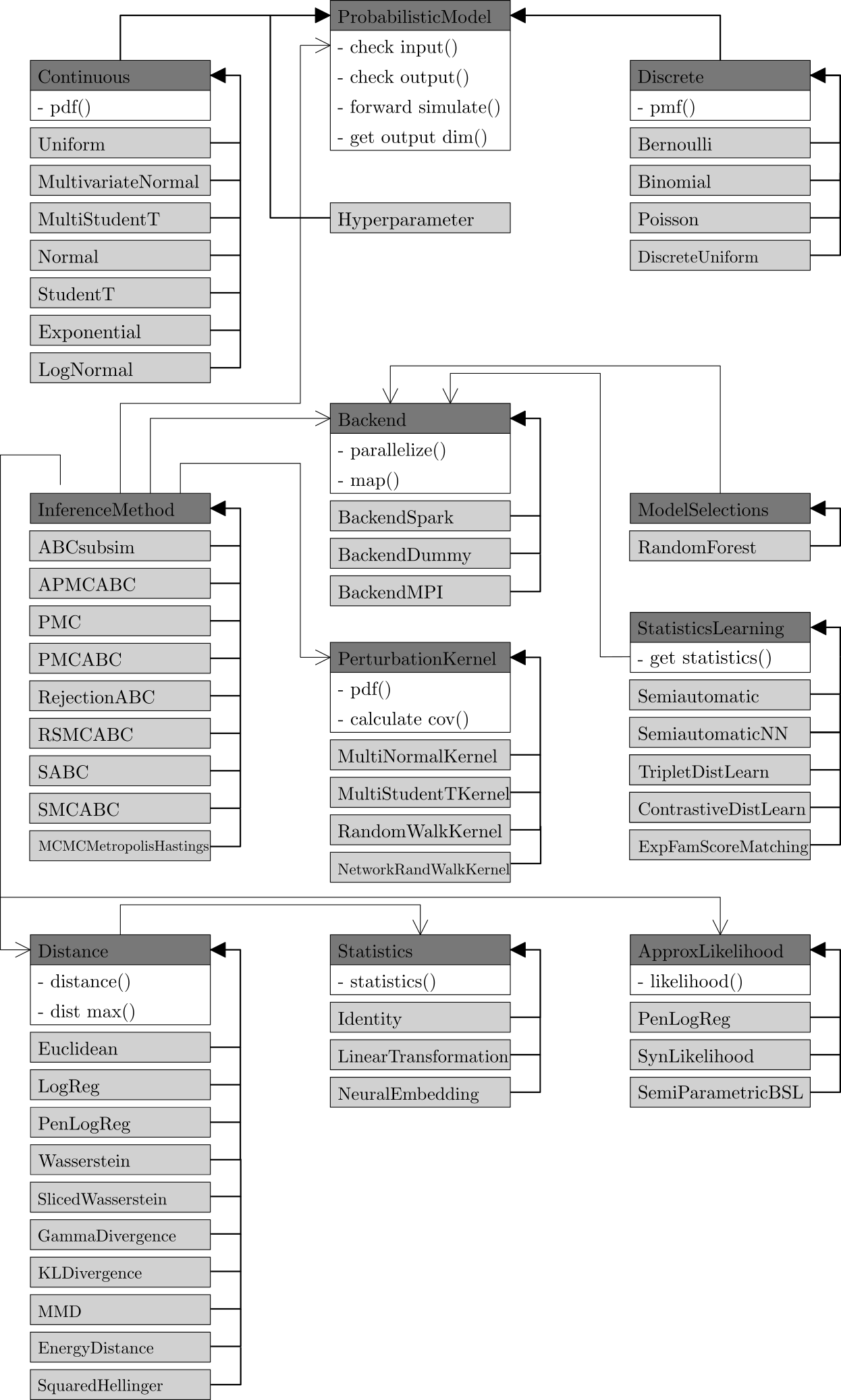
The following diagram shows selected classes with their most important methods. Abstract classes, which cannot be instantiated, are highlighted in dark gray and derived classes are highlighted in light gray. Inheritance is shown by filled arrows. Arrows with no filling highlight associations, e.g., Distance is associated with Statistics because it calls a method of the instantiated class to translate the input data to summary statistics.

abcpy.acceptedparametersmanager module

class abcpy.acceptedparametersmanager.AcceptedParametersManager(model)

Bases: object

__init__(model)

This class manages the accepted parameters and other bds objects.

Parameters:model (list) – List of all root probabilistic models

broadcast(backend, observations)

Broadcasts the observations to observations_bds using the specified backend.

Parameters:

• backend (abcpy.backends object) – The backend used by the inference algorithm
• observations (list) – A list containing all observed data

update_kernel_values(backend, kernel_parameters)

Broadcasts new parameters for each kernel

Parameters:

• backend (abcpy.backends object) – The backend used by the inference algorithm
• kernel_parameters (list) – A list, in which each entry contains the values of the parameters associated with the corresponding kernel in the joint perturbation kernel

update_broadcast(backend, accepted_parameters=None, accepted_weights=None, accepted_cov_mats=None)

Updates the broadcasted values using the specified backend

Parameters:

• backend (abcpy.backend object) – The backend to be used for broadcasting
• accepted_parameters (list) – The accepted parameters to be broadcasted
• accepted_weights (list) – The accepted weights to be broadcasted
• accepted_cov_mats (np.ndarray) – The accepted covariance matrix to be broadcasted

get_mapping(models, is_root=True, index=0)

Returns the order in which the models are discovered during recursive depth-first search. Commonly used when returning the accepted_parameters_bds for certain models.

Parameters:

• models (list) – List of the root probabilistic models of the graph.
• is_root (boolean) – Specifies whether the current list of models is the list of overall root models
• index (integer) – The current index in depth-first search.

Returns:

The first entry corresponds to the mapping of the root model, as well as all its parents. The second entry corresponds to the next index in depth-first search.

Return type:

list

get_accepted_parameters_bds_values(models)

Returns the accepted bds values for the specified models.

Parameters:models (list) – Contains the probabilistic models for which the accepted bds values should be returned Returns:The accepted_parameters_bds values of all the probabilistic models specified in models. Return type:list

abcpy.approx_lhd module

class abcpy.approx_lhd.Approx_likelihood(statistics_calc)

Bases: object

This abstract base class defines the approximate likelihood function.

__init__(statistics_calc)

The constructor of a sub-class must accept a non-optional statistics calculator; then, it must call the __init__ method of the parent class. This ensures that the object is initialized correctly so that the _calculate_summary_stat private method can be called when computing the distances.

Parameters:statistics_calc (abcpy.statistics.Statistics) – Statistics extractor object that conforms to the Statistics class.

loglikelihood(y_obs, y_sim)

To be overwritten by any sub-class: should compute the approximate loglikelihood value given the observed data set y_obs and the data set y_sim simulated from model set at the parameter value.

Parameters:

• y_obs (Python list) – Observed data set.
• y_sim (Python list) – Simulated data set from model at the parameter value.

Returns:

Computed approximate loglikelihood.

Return type:

float

likelihood(y_obs, y_sim)

Computes the likelihood by taking the exponential of the loglikelihood method.

Parameters:

• y_obs (Python list) – Observed data set.
• y_sim (Python list) – Simulated data set from model at the parameter value.

Returns:

Computed approximate likelihood.

Return type:

float

class abcpy.approx_lhd.SynLikelihood(statistics_calc)

Bases: abcpy.approx_lhd.Approx_likelihood

__init__(statistics_calc)

This class implements the approximate likelihood function which computes the approximate likelihood using the synthetic likelihood approach described in Wood [1]. For synthetic likelihood approximation, we compute the robust precision matrix using Ledoit and Wolf’s [2] method.

[1] S. N. Wood. Statistical inference for noisy nonlinear ecological dynamic systems. Nature, 466(7310):1102–1104, Aug. 2010.

[2] O. Ledoit and M. Wolf, A Well-Conditioned Estimator for Large-Dimensional Covariance Matrices, Journal of Multivariate Analysis, Volume 88, Issue 2, pages 365-411, February 2004.

Parameters:statistics_calc (abcpy.statistics.Statistics) – Statistics extractor object that conforms to the Statistics class.

loglikelihood(y_obs, y_sim)

Computes the loglikelihood.

Parameters:

• y_obs (Python list) – Observed data set.
• y_sim (Python list) – Simulated data set from model at the parameter value.

Returns:

Computed approximate loglikelihood.

Return type:

float

class abcpy.approx_lhd.SemiParametricSynLikelihood(statistics_calc, bw_method_marginals='silverman')

Bases: abcpy.approx_lhd.Approx_likelihood

__init__(statistics_calc, bw_method_marginals='silverman')

This class implements the approximate likelihood function which computes the approximate likelihood using the semiparametric Synthetic Likelihood (semiBSL) approach described in [1]. Specifically, this represents the likelihood as a product of univariate marginals and the copula components (exploiting Sklar’s theorem). The marginals are approximated from simulations using a Gaussian KDE, while the copula is assumed to be a Gaussian copula, whose parameters are estimated from data as well.

This does not yet include shrinkage strategies for the correlation matrix.

[1] An, Z., Nott, D. J., & Drovandi, C. (2020). Robust Bayesian synthetic likelihood via a semi-parametric approach. Statistics and Computing, 30(3), 543-557.

Parameters:

• statistics_calc (abcpy.statistics.Statistics) – Statistics extractor object that conforms to the Statistics class.
• bw_method_marginals (str, scalar or callable, optional) – The method used to calculate the estimator bandwidth, passed to scipy.stats.gaussian_kde. Following the docs of that method, this can be ‘scott’, ‘silverman’, a scalar constant or a callable. If a scalar, this will be used directly as kde.factor. If a callable, it should take a gaussian_kde instance as only parameter and return a scalar. If None (default), ‘silverman’ is used. See the Notes in scipy.stats.gaussian_kde for more details.

loglikelihood(y_obs, y_sim)

Computes the loglikelihood. This implementation aims to be equivalent to the BSL R package, but the results are slightly different due to small differences in the way the KDE is performed

Parameters:

• y_obs (Python list) – Observed data set.
• y_sim (Python list) – Simulated data set from model at the parameter value.

Returns:

Computed approximate loglikelihood.

Return type:

float

class abcpy.approx_lhd.PenLogReg(statistics_calc, model, n_simulate, n_folds=10, max_iter=100000, seed=None)

Bases: abcpy.approx_lhd.Approx_likelihood, abcpy.graphtools.GraphTools

__init__(statistics_calc, model, n_simulate, n_folds=10, max_iter=100000, seed=None)

This class implements the approximate likelihood function which computes the approximate likelihood up to a constant using penalized logistic regression described in Dutta et. al. [1]. It takes one additional function handler defining the true model and two additional parameters n_folds and n_simulate correspondingly defining number of folds used to estimate prediction error using cross-validation and the number of simulated dataset sampled from each parameter to approximate the likelihood function. For lasso penalized logistic regression we use glmnet of Friedman et. al. [2].

[1] Thomas, O., Dutta, R., Corander, J., Kaski, S., & Gutmann, M. U. (2020). Likelihood-free inference by ratio estimation. Bayesian Analysis.

[2] Friedman, J., Hastie, T., and Tibshirani, R. (2010). Regularization paths for generalized linear models via coordinate descent. Journal of Statistical Software, 33(1), 1–22.

Parameters:

• statistics_calc (abcpy.statistics.Statistics) – Statistics extractor object that conforms to the Statistics class.
• model (abcpy.models.Model) – Model object that conforms to the Model class.
• n_simulate (int) – Number of data points to simulate for the reference data set; this has to be the same as n_samples_per_param when calling the sampler. The reference data set is generated by drawing parameters from the prior and samples from the model when PenLogReg is instantiated.
• n_folds (int, optional) – Number of folds for cross-validation. The default value is 10.
• max_iter (int, optional) – Maximum passes over the data. The default is 100000.
• seed (int, optional) – Seed for the random number generator. The used glmnet solver is not deterministic, this seed is used for determining the cv folds. The default value is None.

loglikelihood(y_obs, y_sim)

Computes the loglikelihood.

Parameters:

• y_obs (Python list) – Observed data set.
• y_sim (Python list) – Simulated data set from model at the parameter value.

Returns:

Computed approximate loglikelihood.

Return type:

float

abcpy.backends module

class abcpy.backends.base.Backend

Bases: object

This is the base class for every parallelization backend. It essentially resembles the map/reduce API from Spark.

An idea for the future is to implement a MPI version of the backend with the hope to be more complient with standard HPC infrastructure and a potential speed-up.

parallelize(list)

This method distributes the list on the available workers and returns a reference object.

The list should be split into number of workers many parts. Each part should then be sent to a separate worker node.

Parameters:list (Python list) – the list that should get distributed on the worker nodes Returns:A reference object that represents the parallelized list Return type:PDS class (parallel data set)

broadcast(object)

Send object to all worker nodes without splitting it up.

Parameters:object (Python object) – An abitrary object that should be available on all workers Returns:A reference to the broadcasted object Return type:BDS class (broadcast data set)

map(func, pds)

A distributed implementation of map that works on parallel data sets (PDS).

On every element of pds the function func is called.

Parameters:

• func (Python func) – A function that can be applied to every element of the pds
• pds (PDS class) – A parallel data set to which func should be applied

Returns:

a new parallel data set that contains the result of the map

Return type:

PDS class

collect(pds)

Gather the pds from all the workers, send it to the master and return it as a standard Python list.

Parameters:pds (PDS class) – a parallel data set Returns:all elements of pds as a list Return type:Python list

class abcpy.backends.base.PDS

Bases: object

The reference class for parallel data sets (PDS).

__init__()

Initialize self. See help(type(self)) for accurate signature.

class abcpy.backends.base.BDS

Bases: object

The reference class for broadcast data set (BDS).

__init__()

Initialize self. See help(type(self)) for accurate signature.

value()

This method should return the actual object that the broadcast data set represents.

class abcpy.backends.base.BackendDummy

Bases: abcpy.backends.base.Backend

This is a dummy parallelization backend, meaning it doesn’t parallelize anything. It is mainly implemented for testing purpose.

__init__()

Initialize self. See help(type(self)) for accurate signature.

parallelize(python_list)

This actually does nothing: it just wraps the Python list into dummy pds (PDSDummy).

Parameters:python_list (Python list) – Returns: Return type:PDSDummy (parallel data set)

broadcast(object)

This actually does nothing: it just wraps the object into BDSDummy.

Parameters:object (Python object) – Returns: Return type:BDSDummy class

map(func, pds)

This is a wrapper for the Python internal map function.

Parameters:

• func (Python func) – A function that can be applied to every element of the pds
• pds (PDSDummy class) – A pseudo-parallel data set to which func should be applied

Returns:

a new pseudo-parallel data set that contains the result of the map

Return type:

PDSDummy class

collect(pds)

Returns the Python list stored in PDSDummy

Parameters:pds (PDSDummy class) – a pseudo-parallel data set Returns:all elements of pds as a list Return type:Python list

class abcpy.backends.base.PDSDummy(python_list)

Bases: abcpy.backends.base.PDS

This is a wrapper for a Python list to fake parallelization.

__init__(python_list)

Initialize self. See help(type(self)) for accurate signature.

class abcpy.backends.base.BDSDummy(object)

Bases: abcpy.backends.base.BDS

This is a wrapper for a Python object to fake parallelization.

__init__(object)

Initialize self. See help(type(self)) for accurate signature.

value()

This method should return the actual object that the broadcast data set represents.

class abcpy.backends.base.NestedParallelizationController

Bases: object

nested_execution()

run_nested(func, *args, **kwargs)

class abcpy.backends.spark.BackendSpark(sparkContext, parallelism=4)

Bases: abcpy.backends.base.Backend

A parallelization backend for Apache Spark. It is essetially a wrapper for the required Spark functionality.

__init__(sparkContext, parallelism=4)

Initialize the backend with an existing and configured SparkContext.

Parameters:

• sparkContext (pyspark.SparkContext) – an existing and fully configured PySpark context
• parallelism (int) – defines on how many workers a distributed dataset can be distributed

parallelize(python_list)

This is a wrapper of pyspark.SparkContext.parallelize().

Parameters:list (Python list) – list that is distributed on the workers Returns:A reference object that represents the parallelized list Return type:PDSSpark class (parallel data set)

broadcast(object)

This is a wrapper for pyspark.SparkContext.broadcast().

Parameters:object (Python object) – An abitrary object that should be available on all workers Returns:A reference to the broadcasted object Return type:BDSSpark class (broadcast data set)

map(func, pds)

This is a wrapper for pyspark.rdd.map()

Parameters:

• func (Python func) – A function that can be applied to every element of the pds
• pds (PDSSpark class) – A parallel data set to which func should be applied

Returns:

a new parallel data set that contains the result of the map

Return type:

PDSSpark class

collect(pds)

A wrapper for pyspark.rdd.collect()

Parameters:pds (PDSSpark class) – a parallel data set Returns:all elements of pds as a list Return type:Python list

class abcpy.backends.spark.PDSSpark(rdd)

Bases: abcpy.backends.base.PDS

This is a wrapper for Apache Spark RDDs.

__init__(rdd)

Returns:rdd – initialize with an Spark RDD Return type:pyspark.rdd

class abcpy.backends.spark.BDSSpark(bcv)

Bases: abcpy.backends.base.BDS

This is a wrapper for Apache Spark Broadcast variables.

__init__(bcv)

Parameters:bcv (pyspark.broadcast.Broadcast) – Initialize with a Spark broadcast variable

value()

Returns:returns the referenced object that was broadcasted. Return type:object

abcpy.continuousmodels module

class abcpy.continuousmodels.Uniform(parameters, name='Uniform')

Bases: abcpy.probabilisticmodels.ProbabilisticModel, abcpy.probabilisticmodels.Continuous

__init__(parameters, name='Uniform')

This class implements a probabilistic model following an uniform distribution.

Parameters:

• parameters (list) – Contains two lists. The first list specifies the probabilistic models and hyperparameters from which the lower bound of the uniform distribution derive. The second list specifies the probabilistic models and hyperparameters from which the upper bound derives.
• name (string, optional) – The name that should be given to the probabilistic model in the journal file.

forward_simulate(input_values, k, rng=<MagicMock name='mock.RandomState()' id='140064215897104'>, mpi_comm=None)

Samples from a uniform distribution using the current values for each probabilistic model from which the model derives.

Parameters:

• input_values (list) – List of input parameters, in the same order as specified in the InputConnector passed to the init function
• k (integer) – The number of samples that should be drawn.
• rng (Random number generator) – Defines the random number generator to be used. The default value uses a random seed to initialize the generator.

Returns:

list – A list containing the sampled values as np-array.

Return type:

[np.ndarray]

get_output_dimension()

Provides the output dimension of the current model.

This function is in particular important if the current model is used as an input for other models. In such a case it is assumed that the output is always a vector of int or float. The length of the vector is the dimension that should be returned here.

Returns:The dimension of the output vector of a single forward simulation. Return type:int

pdf(input_values, x)

Calculates the probability density function at point x. Commonly used to determine whether perturbed parameters are still valid according to the pdf.

Parameters:

• input_values (list) – List of input parameters, in the same order as specified in the InputConnector passed to the init function
• x (list) – The point at which the pdf should be evaluated.

Returns:

The evaluated pdf at point x.

Return type:

Float

class abcpy.continuousmodels.Normal(parameters, name='Normal')

Bases: abcpy.probabilisticmodels.ProbabilisticModel, abcpy.probabilisticmodels.Continuous

__init__(parameters, name='Normal')

This class implements a probabilistic model following a normal distribution with mean mu and variance sigma.

Parameters:

• parameters (list) – Contains the probabilistic models and hyperparameters from which the model derives. The list has two entries: from the first entry mean of the distribution and from the second entry variance is derived. Note that the second value of the list is strictly greater than 0.
• name (string) – The name that should be given to the probabilistic model in the journal file.

forward_simulate(input_values, k, rng=<MagicMock name='mock.RandomState()' id='140064215472144'>, mpi_comm=None)

Samples from a normal distribution using the current values for each probabilistic model from which the model derives.

Parameters:

• input_values (list) – List of input parameters, in the same order as specified in the InputConnector passed to the init function
• k (integer) – The number of samples that should be drawn.
• rng (Random number generator) – Defines the random number generator to be used. The default value uses a random seed to initialize the generator.

Returns:

list – A list containing the sampled values as np-array.

Return type:

[np.ndarray]

get_output_dimension()

Provides the output dimension of the current model.

This function is in particular important if the current model is used as an input for other models. In such a case it is assumed that the output is always a vector of int or float. The length of the vector is the dimension that should be returned here.

Returns:The dimension of the output vector of a single forward simulation. Return type:int

pdf(input_values, x)

Calculates the probability density function at point x. Commonly used to determine whether perturbed parameters are still valid according to the pdf.

Parameters:

• input_values (list) – List of input parameters of the from [mu, sigma]
• x (list) – The point at which the pdf should be evaluated.

Returns:

The evaluated pdf at point x.

Return type:

Float

class abcpy.continuousmodels.StudentT(parameters, name='StudentT')

Bases: abcpy.probabilisticmodels.ProbabilisticModel, abcpy.probabilisticmodels.Continuous

__init__(parameters, name='StudentT')

This class implements a probabilistic model following the Student’s T-distribution.

Parameters:

• parameters (list) – Contains the probabilistic models and hyperparameters from which the model derives. The list has two entries: from the first entry mean of the distribution and from the second entry degrees of freedom is derived. Note that the second value of the list is strictly greater than 0.
• name (string) – The name that should be given to the probabilistic model in the journal file.

forward_simulate(input_values, k, rng=<MagicMock name='mock.RandomState()' id='140064215109968'>, mpi_comm=None)

Samples from a Student’s T-distribution using the current values for each probabilistic model from which the model derives.

Parameters:

• input_values (list) – List of input parameters, in the same order as specified in the InputConnector passed to the init function
• k (integer) – The number of samples that should be drawn.
• rng (Random number generator) – Defines the random number generator to be used. The default value uses a random seed to initialize the generator.

Returns:

list – A list containing the sampled values as np-array.

Return type:

[np.ndarray]

get_output_dimension()

Provides the output dimension of the current model.

This function is in particular important if the current model is used as an input for other models. In such a case it is assumed that the output is always a vector of int or float. The length of the vector is the dimension that should be returned here.

Returns:The dimension of the output vector of a single forward simulation. Return type:int

pdf(input_values, x)

Calculates the probability density function at point x. Commonly used to determine whether perturbed parameters are still valid according to the pdf.

Parameters:

• input_values (list) – List of input parameters
• x (list) – The point at which the pdf should be evaluated.

Returns:

The evaluated pdf at point x.

Return type:

Float

class abcpy.continuousmodels.MultivariateNormal(parameters, name='Multivariate Normal')

Bases: abcpy.probabilisticmodels.ProbabilisticModel, abcpy.probabilisticmodels.Continuous

__init__(parameters, name='Multivariate Normal')

This class implements a probabilistic model following a multivariate normal distribution with mean and covariance matrix.

Parameters:

• parameters (list of at length 2) – Contains the probabilistic models and hyperparameters from which the model derives. The first entry defines the mean, while the second entry defines the Covariance matrix. Note that if the mean is n dimensional, the covariance matrix is required to be of dimension nxn, symmetric and positive-definite.
• name (string) – The name that should be given to the probabilistic model in the journal file.

forward_simulate(input_values, k, rng=<MagicMock name='mock.RandomState()' id='140064215214672'>, mpi_comm=None)

Samples from a multivariate normal distribution using the current values for each probabilistic model from which the model derives.

Parameters:

• input_values (list) – List of input parameters, in the same order as specified in the InputConnector passed to the init function
• k (integer) – The number of samples that should be drawn.
• rng (Random number generator) – Defines the random number generator to be used. The default value uses a random seed to initialize the generator.

Returns:

list – A list containing the sampled values as np-array.

Return type:

[np.ndarray]

get_output_dimension()

Provides the output dimension of the current model.

This function is in particular important if the current model is used as an input for other models. In such a case it is assumed that the output is always a vector of int or float. The length of the vector is the dimension that should be returned here.

Returns:The dimension of the output vector of a single forward simulation. Return type:int

pdf(input_values, x)

Calculates the probability density function at point x. Commonly used to determine whether perturbed parameters are still valid according to the pdf.

Parameters:

• input_values (list) – List of input parameters
• x (list) – The point at which the pdf should be evaluated.

Returns:

The evaluated pdf at point x.

Return type:

Float

class abcpy.continuousmodels.MultiStudentT(parameters, name='MultiStudentT')

Bases: abcpy.probabilisticmodels.ProbabilisticModel, abcpy.probabilisticmodels.Continuous

__init__(parameters, name='MultiStudentT')

This class implements a probabilistic model following the multivariate Student-T distribution.

Parameters:

• parameters (list) – All but the last two entries contain the probabilistic models and hyperparameters from which the model derives. The second to last entry contains the covariance matrix. If the mean is of dimension n, the covariance matrix is required to be nxn dimensional. The last entry contains the degrees of freedom.
• name (string) – The name that should be given to the probabilistic model in the journal file.

forward_simulate(input_values, k, rng=<MagicMock name='mock.RandomState()' id='140064218781392'>, mpi_comm=None)

Samples from a multivariate Student’s T-distribution using the current values for each probabilistic model from which the model derives.

Parameters:

• input_values (list) – List of input parameters, in the same order as specified in the InputConnector passed to the init function
• k (integer) – The number of samples that should be drawn.
• rng (Random number generator) – Defines the random number generator to be used. The default value uses a random seed to initialize the generator.

Returns:

list – A list containing the sampled values as np-array.

Return type:

[np.ndarray]

get_output_dimension()

Provides the output dimension of the current model.

This function is in particular important if the current model is used as an input for other models. In such a case it is assumed that the output is always a vector of int or float. The length of the vector is the dimension that should be returned here.

Returns:The dimension of the output vector of a single forward simulation. Return type:int

pdf(input_values, x)

Calculates the probability density function at point x. Commonly used to determine whether perturbed parameters are still valid according to the pdf.

Parameters:

• input_values (list) – List of input parameters
• x (list) – The point at which the pdf should be evaluated.

Returns:

The evaluated pdf at point x.

Return type:

Float

class abcpy.continuousmodels.LogNormal(parameters, name='LogNormal')

Bases: abcpy.probabilisticmodels.ProbabilisticModel, abcpy.probabilisticmodels.Continuous

__init__(parameters, name='LogNormal')

This class implements a probabilistic model following a Lognormal distribution with mean mu and variance sigma.

Parameters:

• parameters (list) – Contains the probabilistic models and hyperparameters from which the model derives. The list has two entries: from the first entry mean of the underlying normal distribution and from the second entry variance of the underlying normal distribution is derived. Note that the second value of the list is strictly greater than 0.
• name (string) – The name that should be given to the probabilistic model in the journal file.

forward_simulate(input_values, k, rng=<MagicMock name='mock.RandomState()' id='140064215272848'>, mpi_comm=None)

Samples from a normal distribution using the current values for each probabilistic model from which the model derives.

Parameters:

• input_values (list) – List of input parameters, in the same order as specified in the InputConnector passed to the init function
• k (integer) – The number of samples that should be drawn.
• rng (Random number generator) – Defines the random number generator to be used. The default value uses a random seed to initialize the generator.

Returns:

list – A list containing the sampled values as np-array.

Return type:

[np.ndarray]

get_output_dimension()

Provides the output dimension of the current model.

This function is in particular important if the current model is used as an input for other models. In such a case it is assumed that the output is always a vector of int or float. The length of the vector is the dimension that should be returned here.

Returns:The dimension of the output vector of a single forward simulation. Return type:int

pdf(input_values, x)

Calculates the probability density function at point x. Commonly used to determine whether perturbed parameters are still valid according to the pdf.

Parameters:

• input_values (list) – List of input parameters of the from [mu, sigma]
• x (list) – The point at which the pdf should be evaluated.

Returns:

The evaluated pdf at point x.

Return type:

Float

class abcpy.continuousmodels.Exponential(parameters, name='Exponential')

Bases: abcpy.probabilisticmodels.ProbabilisticModel, abcpy.probabilisticmodels.Continuous

__init__(parameters, name='Exponential')

This class implements a probabilistic model following a normal distribution with mean mu and variance sigma.

Parameters:

• parameters (list) – Contains the probabilistic models and hyperparameters from which the model derives. The list has one entry: the rate \(\lambda\) of the exponential distribution, that has therefore pdf: \(f(x; \lambda) = \lambda \exp(-\lambda x )\)
• name (string) – The name that should be given to the probabilistic model in the journal file.

forward_simulate(input_values, k, rng=<MagicMock name='mock.RandomState()' id='140064215316432'>, mpi_comm=None)

Samples from a normal distribution using the current values for each probabilistic model from which the model derives.

Parameters:

• input_values (list) – List of input parameters, in the same order as specified in the InputConnector passed to the init function
• k (integer) – The number of samples that should be drawn.
• rng (Random number generator) – Defines the random number generator to be used. The default value uses a random seed to initialize the generator.

Returns:

list – A list containing the sampled values as np-array.

Return type:

[np.ndarray]

get_output_dimension()

Provides the output dimension of the current model.

This function is in particular important if the current model is used as an input for other models. In such a case it is assumed that the output is always a vector of int or float. The length of the vector is the dimension that should be returned here.

Returns:The dimension of the output vector of a single forward simulation. Return type:int

pdf(input_values, x)

Calculates the probability density function at point x. Commonly used to determine whether perturbed parameters are still valid according to the pdf.

Parameters:

• input_values (list) – List of input parameters of the from [rate]
• x (list) – The point at which the pdf should be evaluated.

Returns:

The evaluated pdf at point x.

Return type:

Float

abcpy.discretemodels module

class abcpy.discretemodels.Bernoulli(parameters, name='Bernoulli')

Bases: abcpy.probabilisticmodels.Discrete, abcpy.probabilisticmodels.ProbabilisticModel

__init__(parameters, name='Bernoulli')

This class implements a probabilistic model following a bernoulli distribution.

Parameters:

• parameters (list) – A list containing one entry, the probability of the distribution.
• name (string) – The name that should be given to the probabilistic model in the journal file.

forward_simulate(input_values, k, rng=<MagicMock name='mock.RandomState()' id='140064212776272'>, mpi_comm=None)

Samples from the bernoulli distribution associtated with the probabilistic model.

Parameters:

• input_values (list) – List of input parameters, in the same order as specified in the InputConnector passed to the init function
• k (integer) – The number of samples to be drawn.
• rng (random number generator) – The random number generator to be used.

Returns:

list – A list containing the sampled values as np-array.

Return type:

[np.ndarray]

get_output_dimension()

Provides the output dimension of the current model.

This function is in particular important if the current model is used as an input for other models. In such a case it is assumed that the output is always a vector of int or float. The length of the vector is the dimension that should be returned here.

Returns:The dimension of the output vector of a single forward simulation. Return type:int

pmf(input_values, x)

Evaluates the probability mass function at point x.

Parameters:

• input_values (list) – List of input parameters, in the same order as specified in the InputConnector passed to the init function
• x (float) – The point at which the pmf should be evaluated.

Returns:

The pmf evaluated at point x.

Return type:

float

class abcpy.discretemodels.Binomial(parameters, name='Binomial')

Bases: abcpy.probabilisticmodels.Discrete, abcpy.probabilisticmodels.ProbabilisticModel

__init__(parameters, name='Binomial')

This class implements a probabilistic model following a binomial distribution.

Parameters:

• parameters (list) – Contains the probabilistic models and hyperparameters from which the model derives. Note that the first entry of the list, n, an integer and has to be larger than or equal to 0, while the second entry, p, has to be in the interval [0,1].
• name (string) – The name that should be given to the probabilistic model in the journal file.

forward_simulate(input_values, k, rng=<MagicMock name='mock.RandomState()' id='140064212611792'>, mpi_comm=None)

Samples from a binomial distribution using the current values for each probabilistic model from which the model derives.

Parameters:

• input_values (list) – List of input parameters, in the same order as specified in the InputConnector passed to the init function
• k (integer) – The number of samples that should be drawn.
• rng (Random number generator) – Defines the random number generator to be used. The default value uses a random seed to initialize the generator.

Returns:

list – A list containing the sampled values as np-array.

Return type:

[np.ndarray]

get_output_dimension()

Provides the output dimension of the current model.

This function is in particular important if the current model is used as an input for other models. In such a case it is assumed that the output is always a vector of int or float. The length of the vector is the dimension that should be returned here.

Returns:The dimension of the output vector of a single forward simulation. Return type:int

pmf(input_values, x)

Calculates the probability mass function at point x.

Parameters:

• input_values (list) – List of input parameters, in the same order as specified in the InputConnector passed to the init function
• x (list) – The point at which the pmf should be evaluated.

Returns:

The evaluated pmf at point x.

Return type:

Float

class abcpy.discretemodels.Poisson(parameters, name='Poisson')

Bases: abcpy.probabilisticmodels.Discrete, abcpy.probabilisticmodels.ProbabilisticModel

__init__(parameters, name='Poisson')

This class implements a probabilistic model following a poisson distribution.

Parameters:

• parameters (list) – A list containing one entry, the mean of the distribution.
• name (string) – The name that should be given to the probabilistic model in the journal file.

forward_simulate(input_values, k, rng=<MagicMock name='mock.RandomState()' id='140064212634640'>, mpi_comm=None)

Samples k values from the defined possion distribution.

Parameters:

• input_values (list) – List of input parameters, in the same order as specified in the InputConnector passed to the init function
• k (integer) – The number of samples.
• rng (random number generator) – The random number generator to be used.

Returns:

list – A list containing the sampled values as np-array.

Return type:

[np.ndarray]

get_output_dimension()

Provides the output dimension of the current model.

This function is in particular important if the current model is used as an input for other models. In such a case it is assumed that the output is always a vector of int or float. The length of the vector is the dimension that should be returned here.

Returns:The dimension of the output vector of a single forward simulation. Return type:int

pmf(input_values, x)

Calculates the probability mass function of the distribution at point x.

Parameters:

• input_values (list) – List of input parameters, in the same order as specified in the InputConnector passed to the init function
• x (integer) – The point at which the pmf should be evaluated.

Returns:

The evaluated pmf at point x.

Return type:

Float

class abcpy.discretemodels.DiscreteUniform(parameters, name='DiscreteUniform')

Bases: abcpy.probabilisticmodels.Discrete, abcpy.probabilisticmodels.ProbabilisticModel

__init__(parameters, name='DiscreteUniform')

This class implements a probabilistic model following a Discrete Uniform distribution.

Parameters:

• parameters (list) – A list containing two entries, the upper and lower bound of the range.
• name (string) – The name that should be given to the probabilistic model in the journal file.

forward_simulate(input_values, k, rng=<MagicMock name='mock.RandomState()' id='140064214748112'>)

Samples from the Discrete Uniform distribution associated with the probabilistic model.

Parameters:

• input_values (list) – List of input parameters, in the same order as specified in the InputConnector passed to the init function
• k (integer) – The number of samples to be drawn.
• rng (random number generator) – The random number generator to be used.

Returns:

list – A list containing the sampled values as np-array.

Return type:

[np.ndarray]

get_output_dimension()

Provides the output dimension of the current model.

This function is in particular important if the current model is used as an input for other models. In such a case it is assumed that the output is always a vector of int or float. The length of the vector is the dimension that should be returned here.

Returns:The dimension of the output vector of a single forward simulation. Return type:int

pmf(input_values, x)

Evaluates the probability mass function at point x.

Parameters:

• input_values (list) – List of input parameters, in the same order as specified in the InputConnector passed to the init function
• x (float) – The point at which the pmf should be evaluated.

Returns:

The pmf evaluated at point x.

Return type:

float

abcpy.distances module

class abcpy.distances.Distance(statistics_calc)

Bases: object

This abstract base class defines how the distance between the observed and simulated data should be implemented.

__init__(statistics_calc)

The constructor of a sub-class must accept a non-optional statistics calculator as a parameter; then, it must call the __init__ method of the parent class. This ensures that the object is initialized correctly so that the _calculate_summary_stat private method can be called when computing the distances.

Parameters:statistics_calc (abcpy.statistics.Statistics) – Statistics extractor object that conforms to the Statistics class.

distance(d1, d2)

To be overwritten by any sub-class: should calculate the distance between two sets of data d1 and d2 using their respective statistics.

Usually, calling the _calculate_summary_stat private method to obtain statistics from the datasets is handy; that also keeps track of the first provided dataset (which is the observation in ABCpy inference schemes) and avoids computing the statistics for that multiple times.

Notes

The data sets d1 and d2 are array-like structures that contain n1 and n2 data points each. An implementation of the distance function should work along the following steps:

1. Transform both input sets dX = [ dX1, dX2, …, dXn ] to sX = [sX1, sX2, …, sXn] using the statistics object. See _calculate_summary_stat method.

2. Calculate the mutual desired distance, here denoted by - between the statistics; for instance, dist = [s11 - s21, s12 - s22, …, s1n - s2n] (in some cases however you may want to compute all pairwise distances between statistics elements.

Important: any sub-class must not calculate the distance between data sets d1 and d2 directly. This is the reason why any sub-class must be initialized with a statistics object.

Parameters:

• d1 (Python list) – Contains n1 data points.
• d2 (Python list) – Contains n2 data points.

Returns:

The distance between the two input data sets.

Return type:

numpy.float

dist_max()

To be overwritten by sub-class: should return maximum possible value of the desired distance function.

Examples

If the desired distance maps to \(\mathbb{R}\), this method should return numpy.inf.

Returns:The maximal possible value of the desired distance function. Return type:numpy.float

class abcpy.distances.Divergence(statistics_calc)

Bases: abcpy.distances.Distance

This is an abstract class which subclasses Distance, and is used as a parent class for all divergence estimators; more specifically, it is used for all Distances which compare the empirical distribution of simulations and observations.

class abcpy.distances.Euclidean(statistics_calc)

Bases: abcpy.distances.Distance

This class implements the Euclidean distance between two vectors.

The maximum value of the distance is np.inf.

Parameters:statistics_calc (abcpy.statistics.Statistics) – Statistics extractor object that conforms to the Statistics class.

__init__(statistics_calc)

The constructor of a sub-class must accept a non-optional statistics calculator as a parameter; then, it must call the __init__ method of the parent class. This ensures that the object is initialized correctly so that the _calculate_summary_stat private method can be called when computing the distances.

Parameters:statistics_calc (abcpy.statistics.Statistics) – Statistics extractor object that conforms to the Statistics class.

distance(d1, d2)

Calculates the distance between two datasets, by computing Euclidean distance between each element of d1 and d2 and taking their average.

Parameters:

• d1 (Python list) – Contains n1 data points.
• d2 (Python list) – Contains n2 data points.

Returns:

The distance between the two input data sets.

Return type:

numpy.float

dist_max()

Returns:The maximal possible value of the desired distance function. Return type:numpy.float

class abcpy.distances.PenLogReg(statistics_calc)

Bases: abcpy.distances.Divergence

This class implements a distance measure based on the classification accuracy.

The classification accuracy is calculated between two dataset d1 and d2 using lasso penalized logistics regression and return it as a distance. The lasso penalized logistic regression is done using glmnet package of Friedman et. al. [2]. While computing the distance, the algorithm automatically chooses the most relevant summary statistics as explained in Gutmann et. al. [1]. The maximum value of the distance is 1.0.

[1] Gutmann, M. U., Dutta, R., Kaski, S., & Corander, J. (2018). Likelihood-free inference via classification. Statistics and Computing, 28(2), 411-425.

[2] Friedman, J., Hastie, T., and Tibshirani, R. (2010). Regularization paths for generalized linear models via coordinate descent. Journal of Statistical Software, 33(1), 1–22.

Parameters:statistics_calc (abcpy.statistics.Statistics) – Statistics extractor object that conforms to the Statistics class.

__init__(statistics_calc)

The constructor of a sub-class must accept a non-optional statistics calculator as a parameter; then, it must call the __init__ method of the parent class. This ensures that the object is initialized correctly so that the _calculate_summary_stat private method can be called when computing the distances.

Parameters:statistics_calc (abcpy.statistics.Statistics) – Statistics extractor object that conforms to the Statistics class.

distance(d1, d2)

Calculates the distance between two datasets.

Parameters:

• d1 (Python list) – Contains n1 data points.
• d2 (Python list) – Contains n2 data points.

Returns:

The distance between the two input data sets.

Return type:

numpy.float

dist_max()

Returns:The maximal possible value of the desired distance function. Return type:numpy.float

class abcpy.distances.LogReg(statistics_calc, seed=None)

Bases: abcpy.distances.Divergence

This class implements a distance measure based on the classification accuracy [1]. The classification accuracy is calculated between two dataset d1 and d2 using logistics regression and return it as a distance. The maximum value of the distance is 1.0. The logistic regression may not converge when using one single sample in each dataset (as for instance by putting n_samples_per_param=1 in an inference routine).

[1] Gutmann, M. U., Dutta, R., Kaski, S., & Corander, J. (2018). Likelihood-free inference via classification. Statistics and Computing, 28(2), 411-425.

Parameters:

• statistics_calc (abcpy.statistics.Statistics) – Statistics extractor object that conforms to the Statistics class.
• seed (integer, optionl) – Seed used to initialize the Random Numbers Generator used to determine the (random) cross validation split in the Logistic Regression classifier.

__init__(statistics_calc, seed=None)

The constructor of a sub-class must accept a non-optional statistics calculator as a parameter; then, it must call the __init__ method of the parent class. This ensures that the object is initialized correctly so that the _calculate_summary_stat private method can be called when computing the distances.

Parameters:statistics_calc (abcpy.statistics.Statistics) – Statistics extractor object that conforms to the Statistics class.

distance(d1, d2)

Calculates the distance between two datasets.

Parameters:

• d1 (Python list) – Contains n1 data points.
• d2 (Python list) – Contains n2 data points.

Returns:

The distance between the two input data sets.

Return type:

numpy.float

dist_max()

Returns:The maximal possible value of the desired distance function. Return type:numpy.float

class abcpy.distances.Wasserstein(statistics_calc, num_iter_max=100000)

Bases: abcpy.distances.Divergence

This class implements a distance measure based on the 2-Wasserstein distance, as used in [1]. This considers the several simulations/observations in the datasets as iid samples from the model for a fixed parameter value/from the data generating model, and computes the 2-Wasserstein distance between the empirical distributions those simulations/observations define.

[1] Bernton, E., Jacob, P.E., Gerber, M. and Robert, C.P. (2019), Approximate Bayesian computation with the Wasserstein distance. J. R. Stat. Soc. B, 81: 235-269. doi:10.1111/rssb.12312

Parameters:

• statistics_calc (abcpy.statistics.Statistics) – Statistics extractor object that conforms to the Statistics class.
• num_iter_max (integer, optional) – The maximum number of iterations in the linear programming algorithm to estimate the Wasserstein distance. Default to 100000.

__init__(statistics_calc, num_iter_max=100000)

The constructor of a sub-class must accept a non-optional statistics calculator as a parameter; then, it must call the __init__ method of the parent class. This ensures that the object is initialized correctly so that the _calculate_summary_stat private method can be called when computing the distances.

Parameters:statistics_calc (abcpy.statistics.Statistics) – Statistics extractor object that conforms to the Statistics class.

distance(d1, d2)

Calculates the distance between two datasets.

Parameters:

• d1 (Python list) – Contains n1 data points.
• d2 (Python list) – Contains n2 data points.

Returns:

The distance between the two input data sets.

Return type:

numpy.float

dist_max()

Returns:The maximal possible value of the desired distance function. Return type:numpy.float

class abcpy.distances.SlicedWasserstein(statistics_calc, n_projections=50, rng=<MagicMock name='mock.RandomState()' id='140064212041424'>)

Bases: abcpy.distances.Divergence

This class implements a distance measure based on the sliced 2-Wasserstein distance, as used in [1]. This considers the several simulations/observations in the datasets as iid samples from the model for a fixed parameter value/from the data generating model, and computes the sliced 2-Wasserstein distance between the empirical distributions those simulations/observations define. Specifically, the sliced Wasserstein distance is a cheaper version of the Wasserstein distance which consists of projecting the multivariate data on 1d directions and computing the 1d Wasserstein distance, which is computationally cheap. The resulting sliced Wasserstein distance is obtained by averaging over a given number of projections.

[1] Nadjahi, K., De Bortoli, V., Durmus, A., Badeau, R., & Şimşekli, U. (2020, May). Approximate bayesian computation with the sliced-wasserstein distance. In ICASSP 2020-2020 IEEE International Conference on Acoustics, Speech and Signal Processing (ICASSP) (pp. 5470-5474). IEEE.

Parameters:

• statistics_calc (abcpy.statistics.Statistics) – Statistics extractor object that conforms to the Statistics class.
• n_projections (int, optional) – Number of 1d projections used for estimating the sliced Wasserstein distance. Default value is 50.
• rng (np.random.RandomState, optional) – random number generators used to generate the projections. If not provided, a new one is instantiated.

__init__(statistics_calc, n_projections=50, rng=<MagicMock name='mock.RandomState()' id='140064212041424'>)

The constructor of a sub-class must accept a non-optional statistics calculator as a parameter; then, it must call the __init__ method of the parent class. This ensures that the object is initialized correctly so that the _calculate_summary_stat private method can be called when computing the distances.

Parameters:statistics_calc (abcpy.statistics.Statistics) – Statistics extractor object that conforms to the Statistics class.

distance(d1, d2)

Calculates the distance between two datasets.

Parameters:

• d1 (Python list) – Contains n1 data points.
• d2 (Python list) – Contains n2 data points.

Returns:

The distance between the two input data sets.

Return type:

numpy.float

dist_max()

Returns:The maximal possible value of the desired distance function. Return type:numpy.float

static get_random_projections(n_projections, d, seed=None)

Taken from

https://github.com/PythonOT/POT/blob/78b44af2434f494c8f9e4c8c91003fbc0e1d4415/ot/sliced.py

Author: Adrien Corenflos <adrien.corenflos@aalto.fi>

License: MIT License

Generates n_projections samples from the uniform on the unit sphere of dimension d-1: \(\mathcal{U}(\mathcal{S}^{d-1})\)

Parameters:

• n_projections (int) – number of samples requested
• d (int) – dimension of the space
• seed (int or RandomState, optional) – Seed used for numpy random number generator

Returns:

out – The uniform unit vectors on the sphere

Return type:

ndarray, shape (n_projections, d)

Examples

>>> n_projections = 100
>>> d = 5
>>> projs = get_random_projections(n_projections, d)
>>> np.allclose(np.sum(np.square(projs), 1), 1.)  # doctest: +NORMALIZE_WHITESPACE
True

sliced_wasserstein_distance(X_s, X_t, a=None, b=None, n_projections=50, seed=None, log=False)

Taken from

https://github.com/PythonOT/POT/blob/78b44af2434f494c8f9e4c8c91003fbc0e1d4415/ot/sliced.py

Author: Adrien Corenflos <adrien.corenflos@aalto.fi>

License: MIT License

Computes a Monte-Carlo approximation of the 2-Sliced Wasserstein distance \(\mathcal{SWD}_2(\mu, \nu) = \underset{\theta \sim \mathcal{U}(\mathbb{S}^{d-1})}{\mathbb{E}}[\mathcal{W}_2^2(\theta_\# \mu, \theta_\# \nu)]^{\frac{1}{2}}\) where \(\theta_\# \mu\) stands for the pushforwars of the projection \(\mathbb{R}^d \ni X \mapsto \langle \theta, X \rangle\)

Parameters:

• X_s (ndarray, shape (n_samples_a, dim)) – samples in the source domain
• X_t (ndarray, shape (n_samples_b, dim)) – samples in the target domain
• a (ndarray, shape (n_samples_a,), optional) – samples weights in the source domain
• b (ndarray, shape (n_samples_b,), optional) – samples weights in the target domain
• n_projections (int, optional) – Number of projections used for the Monte-Carlo approximation
• seed (int or RandomState or None, optional) – Seed used for numpy random number generator
• log (bool, optional) – if True, sliced_wasserstein_distance returns the projections used and their associated EMD.

Returns:

• cost (float) – Sliced Wasserstein Cost
• log (dict, optional) – log dictionary return only if log==True in parameters

Examples

>>> n_samples_a = 20
>>> reg = 0.1
>>> X = np.random.normal(0., 1., (n_samples_a, 5))
>>> sliced_wasserstein_distance(X, X, seed=0)  # doctest: +NORMALIZE_WHITESPACE
0.0

References

Bonneel, Nicolas, et al. “Sliced and radon wasserstein barycenters of measures.” Journal of Mathematical Imaging and Vision 51.1 (2015): 22-45

class abcpy.distances.GammaDivergence(statistics_calc, k=1, gam=0.1)

Bases: abcpy.distances.Divergence

This implements an empirical estimator of the gamma-divergence for ABC as suggested in [1]. In [1], the gamma-divergence was proposed as a divergence which is robust to outliers. The estimator is based on a nearest neighbor density estimate. Specifically, this considers the several simulations/observations in the datasets as iid samples from the model for a fixed parameter value/from the data generating model, and estimates the divergence between the empirical distributions those simulations/observations define.

[1] Fujisawa, M., Teshima, T., Sato, I., & Sugiyama, M. γ-ABC: Outlier-robust approximate Bayesian computation based on a robust divergence estimator. In A. Banerjee and K. Fukumizu (Eds.), Proceedings of 24th International Conference on Artificial Intelligence and Statistics (AISTATS2021), Proceedings of Machine Learning Research, vol.130, pp.1783-1791, online, Apr. 13-15, 2021.

Parameters:

• statistics_calc (abcpy.statistics.Statistics) – Statistics extractor object that conforms to the Statistics class.
• k (int, optional) – nearest neighbor number for the density estimate. Default value is 1
• gam (float, optional) – the gamma parameter in the definition of the divergence. Default value is 0.1

__init__(statistics_calc, k=1, gam=0.1)

The constructor of a sub-class must accept a non-optional statistics calculator as a parameter; then, it must call the __init__ method of the parent class. This ensures that the object is initialized correctly so that the _calculate_summary_stat private method can be called when computing the distances.

Parameters:statistics_calc (abcpy.statistics.Statistics) – Statistics extractor object that conforms to the Statistics class.

distance(d1, d2)

Calculates the distance between two datasets.

Parameters:

• d1 (Python list) – Contains n1 data points.
• d2 (Python list) – Contains n2 data points.

Returns:

The distance between the two input data sets.

Return type:

numpy.float

dist_max()

Returns:The maximal possible value of the desired distance function. Return type:numpy.float

static skl_estimator_gamma_q(s1, s2, k=1, gam=0.1)

Gamma-Divergence estimator using scikit-learn’s NearestNeighbours s1: (N_1,D) Sample drawn from distribution P s2: (N_2,D) Sample drawn from distribution Q k: Number of neighbours considered (default 1) return: estimated D(P|Q)

Adapted from code provided by Masahiro Fujisawa (University of Tokyo / RIKEN AIP)

class abcpy.distances.KLDivergence(statistics_calc, k=1)

Bases: abcpy.distances.Divergence

This implements an empirical estimator of the KL divergence for ABC as suggested in [1]. The estimator is based on a nearest neighbor density estimate. Specifically, this considers the several simulations/observations in the datasets as iid samples from the model for a fixed parameter value/from the data generating model, and estimates the divergence between the empirical distributions those simulations/observations define.

[1] Jiang, B. (2018, March). Approximate Bayesian computation with Kullback-Leibler divergence as data discrepancy. In International Conference on Artificial Intelligence and Statistics (pp. 1711-1721). PMLR.

Parameters:

• statistics_calc (abcpy.statistics.Statistics) – Statistics extractor object that conforms to the Statistics class.
• k (int, optional) – nearest neighbor number for the density estimate. Default value is 1

__init__(statistics_calc, k=1)

The constructor of a sub-class must accept a non-optional statistics calculator as a parameter; then, it must call the __init__ method of the parent class. This ensures that the object is initialized correctly so that the _calculate_summary_stat private method can be called when computing the distances.

Parameters:statistics_calc (abcpy.statistics.Statistics) – Statistics extractor object that conforms to the Statistics class.

distance(d1, d2)

Calculates the distance between two datasets.

Parameters:

• d1 (Python list) – Contains n1 data points.
• d2 (Python list) – Contains n2 data points.

Returns:

The distance between the two input data sets.

Return type:

numpy.float

dist_max()

Returns:The maximal possible value of the desired distance function. Return type:numpy.float

static skl_estimator_KL_div(s1, s2, k=1)

Adapted from https://github.com/nhartland/KL-divergence-estimators/blob/5473a23f5f13d7557100504611c57c9225b1a6eb/src/knn_divergence.py

MIT license

KL-Divergence estimator using scikit-learn’s NearestNeighbours

s1: (N_1,D) Sample drawn from distribution P s2: (N_2,D) Sample drawn from distribution Q k: Number of neighbours considered (default 1) return: estimated D(P|Q)

class abcpy.distances.MMD(statistics_calc, kernel='gaussian', biased_estimator=False, **kernel_kwargs)

Bases: abcpy.distances.Divergence

This implements an empirical estimator of the MMD for ABC as suggested in [1]. This class implements a gaussian kernel by default but allows specifying different kernel functions. Notice that the original version in [1] suggested an unbiased estimate, which however can return negative values. We also provide a biased but provably positive estimator following the remarks in [2]. Specifically, this considers the several simulations/observations in the datasets as iid samples from the model for a fixed parameter value/from the data generating model, and estimates the MMD between the empirical distributions those simulations/observations define.

[1] Park, M., Jitkrittum, W., & Sejdinovic, D. (2016, May). K2-ABC: Approximate Bayesian computation with kernel embeddings. In Artificial Intelligence and Statistics (pp. 398-407). PMLR. [2] Nguyen, H. D., Arbel, J., Lü, H., & Forbes, F. (2020). Approximate Bayesian computation via the energy statistic. IEEE Access, 8, 131683-131698.

Parameters:

• statistics_calc (abcpy.statistics.Statistics) – Statistics extractor object that conforms to the Statistics class.
• kernel (str or callable) – Can be a string denoting the kernel, or a function. If a string, only gaussian is implemented for now; in that case, you can also provide an additional keyword parameter ‘sigma’ which is used as the sigma in the kernel. Default is the gaussian kernel.
• biased_estimator (boolean, optional) – Whether to use the biased (but always positive) or unbiased estimator; by default, it uses the biased one.
• kernel_kwargs – Additional keyword arguments to be passed to the distance calculator.

__init__(statistics_calc, kernel='gaussian', biased_estimator=False, **kernel_kwargs)

The constructor of a sub-class must accept a non-optional statistics calculator as a parameter; then, it must call the __init__ method of the parent class. This ensures that the object is initialized correctly so that the _calculate_summary_stat private method can be called when computing the distances.

Parameters:statistics_calc (abcpy.statistics.Statistics) – Statistics extractor object that conforms to the Statistics class.

distance(d1, d2)

Calculates the distance between two datasets.

Parameters:

• d1 (Python list) – Contains n1 data points.
• d2 (Python list) – Contains n2 data points.

Returns:

The distance between the two input data sets.

Return type:

numpy.float

dist_max()

Returns:The maximal possible value of the desired distance function. Return type:numpy.float

static def_gaussian_kernel(sigma=1)

compute_Gram_matrix(s1, s2)

static MMD_unbiased(Kxx, Kyy, Kxy)

static MMD_V_estimator(Kxx, Kyy, Kxy)

class abcpy.distances.EnergyDistance(statistics_calc, base_distance='Euclidean', biased_estimator=True, **base_distance_kwargs)

Bases: abcpy.distances.MMD

This implements an empirical estimator of the Energy Distance for ABC as suggested in [1]. This class uses the Euclidean distance by default as a base distance, but allows to pass different distances. Moreover, when the Euclidean distance is specified, it is possible to pass an additional keyword argument beta which denotes the power of the distance to consider. In [1], the authors suggest to use a biased but provably positive estimator; we also provide an unbiased estimate, which however can return negative values. Specifically, this considers the several simulations/observations in the datasets as iid samples from the model for a fixed parameter value/from the data generating model, and estimates the MMD between the empirical distributions those simulations/observations define.

[1] Nguyen, H. D., Arbel, J., Lü, H., & Forbes, F. (2020). Approximate Bayesian computation via the energy statistic. IEEE Access, 8, 131683-131698.

Parameters:

• statistics_calc (abcpy.statistics.Statistics) – Statistics extractor object that conforms to the Statistics class.
• base_distance (str or callable) – Can be a string denoting the kernel, or a function. If a string, only Euclidean distance is implemented for now; in that case, you can also provide an additional keyword parameter ‘beta’ which is the power of the distance to consider. By default, this uses the Euclidean distance.
• biased_estimator (boolean, optional) – Whether to use the biased (but always positive) or unbiased estimator; by default, it uses the biased one.
• base_distance_kwargs – Additional keyword arguments to be passed to the distance calculator.

__init__(statistics_calc, base_distance='Euclidean', biased_estimator=True, **base_distance_kwargs)

The constructor of a sub-class must accept a non-optional statistics calculator as a parameter; then, it must call the __init__ method of the parent class. This ensures that the object is initialized correctly so that the _calculate_summary_stat private method can be called when computing the distances.

Parameters:statistics_calc (abcpy.statistics.Statistics) – Statistics extractor object that conforms to the Statistics class.

dist_max()

Returns:The maximal possible value of the desired distance function. Return type:numpy.float

static def_Euclidean_distance(beta=1)

class abcpy.distances.SquaredHellingerDistance(statistics_calc, k=1)

Bases: abcpy.distances.Divergence

This implements an empirical estimator of the squared Hellinger distance for ABC. Using the Hellinger distance was suggested originally in [1], but as that work did not provide originally any implementation details, this implementation is original. The estimator is based on a nearest neighbor density estimate. Specifically, this considers the several simulations/observations in the datasets as iid samples from the model for a fixed parameter value/from the data generating model, and estimates the divergence between the empirical distributions those simulations/observations define.

[1] Frazier, D. T. (2020). Robust and Efficient Approximate Bayesian Computation: A Minimum Distance Approach. arXiv preprint arXiv:2006.14126.

Parameters:

• statistics_calc (abcpy.statistics.Statistics) – Statistics extractor object that conforms to the Statistics class.
• k (int, optional) – nearest neighbor number for the density estimate. Default value is 1

__init__(statistics_calc, k=1)

The constructor of a sub-class must accept a non-optional statistics calculator as a parameter; then, it must call the __init__ method of the parent class. This ensures that the object is initialized correctly so that the _calculate_summary_stat private method can be called when computing the distances.

Parameters:statistics_calc (abcpy.statistics.Statistics) – Statistics extractor object that conforms to the Statistics class.

distance(d1, d2)

Calculates the distance between two datasets.

Parameters:

• d1 (Python list) – Contains n1 data points.
• d2 (Python list) – Contains n2 data points.

Returns:

The distance between the two input data sets.

Return type:

numpy.float

dist_max()

Returns:The maximal possible value of the desired distance function. Return type:numpy.float

static skl_estimator_squared_Hellinger_distance(s1, s2, k=1)

Squared Hellinger distance estimator using scikit-learn’s NearestNeighbours s1: (N_1,D) Sample drawn from distribution P s2: (N_2,D) Sample drawn from distribution Q k: Number of neighbours considered (default 1) return: estimated D(P|Q)

abcpy.graphtools module

class abcpy.graphtools.GraphTools

Bases: object

This class implements all methods that will be called recursively on the graph structure.

sample_from_prior(model=None, rng=<MagicMock name='mock.RandomState()' id='140064218810576'>)

Samples values for all random variables of the model. Commonly used to sample new parameter values on the whole graph.

Parameters:

• model (abcpy.ProbabilisticModel object) – The root model for which sample_from_prior should be called.
• rng (Random number generator) – Defines the random number generator to be used

pdf_of_prior(models, parameters, mapping=None, is_root=True)

Calculates the joint probability density function of the prior of the specified models at the given parameter values. Commonly used to check whether new parameters are valid given the prior, as well as to calculate acceptance probabilities.

Parameters:

• models (list of abcpy.ProbabilisticModel objects) – Defines the models for which the pdf of their prior should be evaluated
• parameters (python list) – The parameters at which the pdf should be evaluated
• mapping (list of tuples) – Defines the mapping of probabilistic models and index in a parameter list.
• is_root (boolean) – A flag specifying whether the provided models are the root models. This is to ensure that the pdf is calculated correctly.

Returns:

The resulting pdf,as well as the next index to be considered in the parameters list.

Return type:

list

get_parameters(models=None, is_root=True)

Returns the current values of all free parameters in the model. Commonly used before perturbing the parameters of the model.

Parameters:

• models (list of abcpy.ProbabilisticModel objects) – The models for which, together with their parents, the parameter values should be returned. If no value is provided, the root models are assumed to be the model of the inference method.
• is_root (boolean) – Specifies whether the current models are at the root. This ensures that the values corresponding to simulated observations will not be returned.

Returns:

A list containing all currently sampled values of the free parameters.

Return type:

list

set_parameters(parameters, models=None, index=0, is_root=True)

Sets new values for the currently used values of each random variable. Commonly used after perturbing the parameter values using a kernel.

Parameters:

• parameters (list) – Defines the values to which the respective parameter values of the models should be set
• model (list of abcpy.ProbabilisticModel objects) – Defines all models for which, together with their parents, new values should be set. If no value is provided, the root models are assumed to be the model of the inference method.
• index (integer) – The current index to be considered in the parameters list
• is_root (boolean) – Defines whether the current models are at the root. This ensures that only values corresponding to random variables will be set.

Returns:

list – Returns whether it was possible to set all parameters and the next index to be considered in the parameters list.

Return type:

[boolean, integer]

get_correct_ordering(parameters_and_models, models=None, is_root=True)

Orders the parameters returned by a kernel in the order required by the graph. Commonly used when perturbing the parameters.

Parameters:

• parameters_and_models (list of tuples) – Contains tuples containing as the first entry the probabilistic model to be considered and as the second entry the parameter values associated with this model
• models (list) – Contains the root probabilistic models that make up the graph. If no value is provided, the root models are assumed to be the model of the inference method.

Returns:

The ordering which can be used by recursive functions on the graph.

Return type:

list

simulate(n_samples_per_param, rng=<MagicMock name='mock.RandomState()' id='140064217918416'>, npc=None)

Simulates data of each model using the currently sampled or perturbed parameters.

Parameters:rng (random number generator) – The random number generator to be used. Returns:Each entry corresponds to the simulated data of one model. Return type:list

abcpy.inferences module

abcpy.modelselections module

class abcpy.modelselections.ModelSelections(model_array, statistics_calc, backend, seed=None)

Bases: object

This abstract base class defines a model selection rule of how to choose a model from a set of models given an observation.

__init__(model_array, statistics_calc, backend, seed=None)

Constructor that must be overwritten by the sub-class.

The constructor of a sub-class must accept an array of models to choose the model from, and two non-optional parameters statistics calculator and backend stored in self.statistics_calc and self.backend defining how to calculate sumarry statistics from data and what kind of parallelization to use.

Parameters:

• model_array (list) – A list of models which are of type abcpy.probabilisticmodels
• statistics (abcpy.statistics.Statistics) – Statistics object that conforms to the Statistics class.
• backend (abcpy.backends.Backend) – Backend object that conforms to the Backend class.
• seed (integer, optional) – Optional initial seed for the random number generator. The default value is generated randomly.

select_model(observations, n_samples=1000, n_samples_per_param=100)

To be overwritten by any sub-class: returns a model selected by the modelselection procedure most suitable to the obersved data set observations. Further two optional integer arguments n_samples and n_samples_per_param is supplied denoting the number of samples in the refernce table and the data points in each simulated data set.

Parameters:

• observations (python list) – The observed data set.
• n_samples (integer, optional) – Number of samples to generate for reference table.
• n_samples_per_param (integer, optional) – Number of data points in each simulated data set.

Returns:

A model which are of type abcpy.probabilisticmodels

Return type:

abcpy.probabilisticmodels

posterior_probability(observations)

To be overwritten by any sub-class: returns the approximate posterior probability of the chosen model given the observed data set observations.

Parameters:observations (python list) – The observed data set. Returns:A vector containing the approximate posterior probability of the model chosen. Return type:np.ndarray

class abcpy.modelselections.RandomForest(model_array, statistics_calc, backend, N_tree=100, n_try_fraction=0.5, seed=None)

Bases: abcpy.modelselections.ModelSelections, abcpy.graphtools.GraphTools

This class implements the model selection procedure based on the Random Forest ensemble learner as described in Pudlo et. al. [1].

[1] Pudlo, P., Marin, J.-M., Estoup, A., Cornuet, J.-M., Gautier, M. and Robert, C. (2016). Reliable ABC model choice via random forests. Bioinformatics, 32 859–866.

__init__(model_array, statistics_calc, backend, N_tree=100, n_try_fraction=0.5, seed=None)

Parameters:

• N_tree (integer, optional) – Number of trees in the random forest. The default value is 100.
• n_try_fraction (float, optional) – The fraction of number of summary statistics to be considered as the size of the number of covariates randomly sampled at each node by the randomised CART. The default value is 0.5.

select_model(observations, n_samples=1000, n_samples_per_param=1)

Parameters:

• observations (python list) – The observed data set.
• n_samples (integer, optional) – Number of samples to generate for reference table. The default value is 1000.
• n_samples_per_param (integer, optional) – Number of data points in each simulated data set. The default value is 1.

Returns:

A model which are of type abcpy.probabilisticmodels

Return type:

abcpy.probabilisticmodels

posterior_probability(observations, n_samples=1000, n_samples_per_param=1)

Parameters:observations (python list) – The observed data set. Returns:A vector containing the approximate posterior probability of the model chosen. Return type:np.ndarray

abcpy.NN_utilities module

Functions and classes needed for the neural network based summary statistics learning.

abcpy.NN_utilities.algorithms.contrastive_training(samples, similarity_set, embedding_net, cuda, batch_size=16, n_epochs=200, samples_val=None, similarity_set_val=None, early_stopping=False, epochs_early_stopping_interval=1, start_epoch_early_stopping=10, positive_weight=None, load_all_data_GPU=False, margin=1.0, lr=None, optimizer=None, scheduler=None, start_epoch_training=0, use_tqdm=True, optimizer_kwargs={}, scheduler_kwargs={}, loader_kwargs={})

Implements the algorithm for the contrastive distance learning training of a neural network; need to be provided with a set of samples and the corresponding similarity matrix

abcpy.NN_utilities.algorithms.triplet_training(samples, similarity_set, embedding_net, cuda, batch_size=16, n_epochs=400, samples_val=None, similarity_set_val=None, early_stopping=False, epochs_early_stopping_interval=1, start_epoch_early_stopping=10, load_all_data_GPU=False, margin=1.0, lr=None, optimizer=None, scheduler=None, start_epoch_training=0, use_tqdm=True, optimizer_kwargs={}, scheduler_kwargs={}, loader_kwargs={})

Implements the algorithm for the triplet distance learning training of a neural network; need to be provided with a set of samples and the corresponding similarity matrix

abcpy.NN_utilities.algorithms.FP_nn_training(samples, target, embedding_net, cuda, batch_size=1, n_epochs=50, samples_val=None, target_val=None, early_stopping=False, epochs_early_stopping_interval=1, start_epoch_early_stopping=10, load_all_data_GPU=False, lr=0.001, optimizer=None, scheduler=None, start_epoch_training=0, use_tqdm=True, optimizer_kwargs={}, scheduler_kwargs={}, loader_kwargs={})

Implements the algorithm for the training of a neural network based on regressing the values of the parameters on the corresponding simulation outcomes; it is effectively a training with a mean squared error loss. Needs to be provided with a set of samples and the corresponding parameters that generated the samples. Note that in this case the network has to have same output size as the number of parameters, as the learned summary statistic will have the same dimension as the parameter.

class abcpy.NN_utilities.datasets.Similarities(samples, similarity_matrix, device)

Bases: sphinx.ext.autodoc.importer._MockObject

A dataset class that considers a set of samples and pairwise similarities defined between them. Note that, for our application of computing distances, we are not interested in train/test split.

__init__(samples, similarity_matrix, device)

Parameters:

samples: n_samples x n_features similarity_matrix: n_samples x n_samples

class abcpy.NN_utilities.datasets.SiameseSimilarities(similarities_dataset, positive_weight=None)

Bases: sphinx.ext.autodoc.importer._MockObject

This class defines a dataset returning pairs of similar and dissimilar samples. It has to be instantiated with a dataset of the class Similarities

__init__(similarities_dataset, positive_weight=None)

If positive_weight=None, then for each sample we pick another random element to form a pair. If positive_weight is a number (in [0,1]), we will pick positive samples with that probability (if there are some).

class abcpy.NN_utilities.datasets.TripletSimilarities(similarities_dataset)

Bases: sphinx.ext.autodoc.importer._MockObject

This class defines a dataset returning triplets of anchor, positive and negative samples. It has to be instantiated with a dataset of the class Similarities.

__init__(similarities_dataset)

Initialize self. See help(type(self)) for accurate signature.

class abcpy.NN_utilities.datasets.ParameterSimulationPairs(simulations, parameters, device)

Bases: sphinx.ext.autodoc.importer._MockObject

A dataset class that consists of pairs of parameters-simulation pairs, in which the data contains the simulations, with shape (n_samples, n_features), and targets contains the ground truth of the parameters, with shape (n_samples, 2). Note that n_features could also have more than one dimension here.

__init__(simulations, parameters, device)

Parameters:

simulations: (n_samples, n_features) parameters: (n_samples, 2)

class abcpy.NN_utilities.losses.ContrastiveLoss(margin)

Bases: sphinx.ext.autodoc.importer._MockObject

Contrastive loss Takes embeddings of two samples and a target label == 1 if samples are from the same class and label == 0 otherwise.

Code from https://github.com/adambielski/siamese-triplet

__init__(margin)

Initialize self. See help(type(self)) for accurate signature.

forward(output1, output2, target, size_average=True)

class abcpy.NN_utilities.losses.TripletLoss(margin)

Bases: sphinx.ext.autodoc.importer._MockObject

Triplet loss Takes embeddings of an anchor sample, a positive sample and a negative sample.

Code from https://github.com/adambielski/siamese-triplet

__init__(margin)

Initialize self. See help(type(self)) for accurate signature.

forward(anchor, positive, negative, size_average=True)

abcpy.NN_utilities.losses.Fisher_divergence_loss(first_der_t, second_der_t, eta, lam=0)

lam is the regularization parameter of the Kingma & LeCun (2010) regularization

abcpy.NN_utilities.losses.Fisher_divergence_loss_with_c_x(first_der_t, second_der_t, eta, lam=0)

class abcpy.NN_utilities.networks.SiameseNet(embedding_net)

Bases: sphinx.ext.autodoc.importer._MockObject

This is used in the contrastive distance learning. It is a network wrapping a standard neural network and feeding two samples through it at once.

From https://github.com/adambielski/siamese-triplet

__init__(embedding_net)

Initialize self. See help(type(self)) for accurate signature.

forward(x1, x2)

get_embedding(x)

class abcpy.NN_utilities.networks.TripletNet(embedding_net)

Bases: sphinx.ext.autodoc.importer._MockObject

This is used in the triplet distance learning. It is a network wrapping a standard neural network and feeding three samples through it at once.

From https://github.com/adambielski/siamese-triplet

__init__(embedding_net)

Initialize self. See help(type(self)) for accurate signature.

forward(x1, x2, x3)

get_embedding(x)

class abcpy.NN_utilities.networks.ScalerAndNet(net, scaler)

Bases: sphinx.ext.autodoc.importer._MockObject

Defines a nn.Module class that wraps a scaler and a neural network, and applies the scaler before passing the data through the neural network.

__init__(net, scaler)

forward(x)

class abcpy.NN_utilities.networks.DiscardLastOutputNet(net)

Bases: sphinx.ext.autodoc.importer._MockObject

Defines a nn.Module class that wraps a scaler and a neural network, and applies the scaler before passing the data through the neural network. Next, the

__init__(net)

Initialize self. See help(type(self)) for accurate signature.

forward(x)

abcpy.NN_utilities.networks.createDefaultNN(input_size, output_size, hidden_sizes=None, nonlinearity=None, batch_norm_last_layer=False, batch_norm_last_layer_momentum=0.1)

Function returning a fully connected neural network class with a given input and output size, and optionally given hidden layer sizes (if these are not given, they are determined from the input and output size in a heuristic way, see below).

In order to instantiate the network, you need to write:

>>> createDefaultNN(input_size, output_size)()

as the function returns a class, and () is needed to instantiate an object.

If hidden_sizes is None, three hidden layers are used with the following sizes: [int(input_size * 1.5), int(input_size * 0.75 + output_size * 3), int(output_size * 5)]

Note that the nonlinearity here is as an object or a functional, not a class, eg:

nonlinearity = nn.Softplus()

or:

nonlinearity = nn.functional.softplus

abcpy.NN_utilities.networks.createDefaultNNWithDerivatives(input_size, output_size, hidden_sizes=None, nonlinearity=None, first_derivative_only=False)

Function returning a fully connected neural network class with a given input and output size, and optionally given hidden layer sizes (if these are not given, they are determined from the input and output size with some expression. This neural network is capable of computing the first and second derivatives of output with respect to input along with the forward pass.

All layers in this neural network are linear.

>>> createDefaultNN(input_size, output_size)()

as the function returns a class, and () is needed to instantiate an object.

If hidden_sizes is None, three hidden layers are used with the following sizes: [int(input_size * 1.5), int(input_size * 0.75 + output_size * 3), int(output_size * 5)]

Note that the nonlinearity here is passed as a class, not an object, eg:

nonlinearity = nn.Softplus

abcpy.NN_utilities.utilities.dist2(x, y)

Compute the square of the Euclidean distance between 2 arrays of same length

abcpy.NN_utilities.utilities.compute_similarity_matrix(target, quantile=0.1, return_pairwise_distances=False)

Compute the similarity matrix between some values given a given quantile of the Euclidean distances.

If return_pairwise_distances is True, it also returns a matrix with the pairwise distances with every distance.

abcpy.NN_utilities.utilities.save_net(path, net)

Function to save the Pytorch state_dict of a network to a file.

abcpy.NN_utilities.utilities.load_net(path, network_class, *network_args, **network_kwargs)

Function to load a network from a Pytorch state_dict, given the corresponding network_class.

abcpy.NN_utilities.utilities.jacobian(input, output, diffable=True)

Returns the Jacobian matrix (batch x in_size x out_size) of the function that produced the output evaluated at the input

From https://github.com/mwcvitkovic/MASS-Learning/blob/master/models/utils.py

Important: need to use diffable=True in order for the training routines based on these to work!

abcpy.NN_utilities.utilities.jacobian_second_order(input, output, diffable=True)

Returns the Jacobian matrix (batch x in_size x out_size) of the function that produced the output evaluated at the input, as well as the matrix of second derivatives of outputs with respect to inputs (batch x in_size x out_size)

Adapted from https://github.com/mwcvitkovic/MASS-Learning/blob/master/models/utils.py

Important: need to use diffable=True in order for the training routines based on these to work!

abcpy.NN_utilities.utilities.jacobian_hessian(input, output, diffable=True)

Returns the Jacobian matrix (batch x in_size x out_size) of the function that produced the output evaluated at the input, as well as the Hessian matrix (batch x in_size x in_size x out_size).

This takes slightly more than the jacobian_second_order routine.

Adapted from https://github.com/mwcvitkovic/MASS-Learning/blob/master/models/utils.py

Important: need to use diffable=True in order for the training routines based on these to work!

abcpy.NN_utilities.utilities.set_requires_grad(net, value)

abcpy.output module

class abcpy.output.Journal(type)

Bases: object

The journal holds information created by the run of inference schemes.

It can be configured to even hold intermediate.

accepted_parameters

List of lists containing posterior samples

Type:list

names_and_parameters

List of dictionaries containing posterior samples with parameter names as keys

Type:list

accepted_simulations

List of lists containing simulations corresponding to posterior samples (this could be empty if the sampling routine does not store those)

Type:list

accepted_cov_mats

List of lists containing covariance matrices from accepted posterior samples (this could be empty if the sampling routine does not store those)

Type:list

weights

List containing posterior weights

Type:list

ESS

List containing the Effective Sample Size (ESS) at each iteration

Type:list

distances

List containing the ABC distance at each iteration

Type:list

configuration

dictionary containing the schemes configuration parameters

Type:Python dictionary

__init__(type)

Initializes a new output journal of given type.

Parameters:type (int (identifying type)) – type=0 only logs final parametersa and weight (production use); type=1 logs all generated information (reproducibily use).

classmethod fromFile(filename)

This method reads a saved journal from disk an returns it as an object.

Notes

To store a journal use Journal.save(filename).

Parameters:filename (string) – The string representing the location of a file Returns:The journal object serialized in <filename> Return type:abcpy.output.Journal

Example

>>> jnl = Journal.fromFile('example_output.jnl')

add_user_parameters(names_and_params)

Saves the provided parameters and names of the probabilistic models corresponding to them. If type==0, old parameters get overwritten.

Parameters:names_and_params (list) – Each entry is a tuple, where the first entry is the name of the probabilistic model, and the second entry is the parameters associated with this model.

add_accepted_parameters(accepted_parameters)

FIX THIS! Saves provided accepted parameters by appending them to the journal. If type==0, old accepted parameters get overwritten.

Parameters:accepted_parameters (list) –

add_accepted_simulations(accepted_simulations)

Saves provided accepted simulations by appending them to the journal. If type==0, old accepted simulations get overwritten.

Parameters:accepted_simulations (list) –

add_accepted_cov_mats(accepted_cov_mats)

Saves provided accepted cov_mats by appending them to the journal. If type==0, old accepted cov_mats get overwritten.

Parameters:accepted_cov_mats (list) –

add_weights(weights)

Saves provided weights by appending them to the journal. If type==0, old weights get overwritten.

Parameters:weights (numpy.array) – vector containing n weigths

add_distances(distances)

Saves provided distances by appending them to the journal. If type==0, old weights get overwritten.

Parameters:distances (numpy.array) – vector containing n distances

add_ESS_estimate(weights)

Computes and saves Effective Sample Size (ESS) estimate starting from provided weights; ESS is estimated as sum the inverse of sum of squared normalized weights. The provided weights are normalized before computing ESS. If type==0, old ESS estimate gets overwritten.

Parameters:weights (numpy.array) – vector containing n weigths

save(filename)

Stores the journal to disk.

Parameters:filename (string) – the location of the file to store the current object to.

get_parameters(iteration=None)

Returns the parameters from a sampling scheme.

For intermediate results, pass the iteration.

Parameters:iteration (int) – specify the iteration for which to return parameters Returns:names_and_parameters – Samples from the specified iteration (last, if not specified) returned as a disctionary with names of the random variables Return type:dictionary

get_accepted_parameters(iteration=None)

Returns the accepted parameters from a sampling scheme.

For intermediate results, pass the iteration.

Parameters:iteration (int) – specify the iteration for which to return parameters Returns:accepted_parameters – List containing samples from the specified iteration (last, if not specified) Return type:list

get_accepted_simulations(iteration=None)

Returns the accepted simulations from a sampling scheme. Notice not all sampling schemes store those in the Journal, so this may return None.

For intermediate results, pass the iteration.

Parameters:iteration (int) – specify the iteration for which to return accepted simulations Returns:accepted_simulations – List containing simulations corresponding to accepted samples from the specified iteration (last, if not specified) Return type:list

get_accepted_cov_mats(iteration=None)

Returns the accepted cov_mats used in a sampling scheme. Notice not all sampling schemes store those in the Journal, so this may return None.

For intermediate results, pass the iteration.

Parameters:iteration (int) – specify the iteration for which to return accepted cov_mats Returns:accepted_cov_mats – List containing accepted cov_mats from the specified iteration (last, if not specified) Return type:list

get_weights(iteration=None)

Returns the weights from a sampling scheme.

For intermediate results, pass the iteration.

Parameters:iteration (int) – specify the iteration for which to return weights

get_distances(iteration=None)

Returns the distances from a sampling scheme.

For intermediate results, pass the iteration.

Parameters:iteration (int) – specify the iteration for which to return distances

get_ESS_estimates(iteration=None)

Returns the estimate of Effective Sample Size (ESS) from a sampling scheme.

For intermediate results, pass the iteration.

Parameters:iteration (int) – specify the iteration for which to return ESS

posterior_mean(iteration=None)

Computes posterior mean from the samples drawn from posterior distribution

For intermediate results, pass the iteration.

Parameters:iteration (int) – specify the iteration for which to return posterior mean Returns:posterior mean – Posterior mean from the specified iteration (last, if not specified) returned as a disctionary with names of the random variables Return type:dictionary

posterior_cov(iteration=None)

Computes posterior covariance from the samples drawn from posterior distribution

Returns:

• np.ndarray – posterior covariance
• dic – order of the variables in the covariance matrix

posterior_histogram(iteration=None, n_bins=10)

Computes a weighted histogram of multivariate posterior samples and returns histogram H and a list of p arrays describing the bin edges for each dimension.

Returns:containing two elements (H = np.ndarray, edges = list of p arrays) Return type:python list

plot_posterior_distr(parameters_to_show=None, ranges_parameters=None, iteration=None, show_samples=None, single_marginals_only=False, double_marginals_only=False, write_posterior_mean=True, show_posterior_mean=True, true_parameter_values=None, contour_levels=14, figsize=None, show_density_values=True, bw_method=None, path_to_save=None)

Produces a visualization of the posterior distribution of the parameters of the model.

A Gaussian kernel density estimate (KDE) is used to approximate the density starting from the sampled parameters. Specifically, it produces a scatterplot matrix, where the diagonal contains single parameter marginals, while the off diagonal elements contain the contourplot for the paired marginals for each possible pair of parameters.

This visualization is not satisfactory for parameters that take on discrete values, specially in the case where the number of values it can assume are small, as it obtains the posterior by KDE in this case as well. We need to improve on that, considering histograms.

Parameters:

• parameters_to_show (list, optional) – a list of the parameters for which you want to plot the posterior distribution. For each parameter, you need to provide the name string as it was defined in the model. For instance, jrnl.plot_posterior_distr(parameters_to_show=[“mu”]) will only plot the posterior distribution for the parameter named “mu” in the list of parameters. If None, then all parameters will be displayed.
• ranges_parameters (Python dictionary, optional) – a dictionary in which you can optionally provide the plotting range for the parameters that you chose to display. You can use this even if parameters_to_show=None. The dictionary key is the name of parameter, and the range needs to be an array-like of the form [lower_limit, upper_limit]. For instance: {“theta” : [0,2]} specifies that you want to plot the posterior distribution for the parameter “theta” in the range [0,2].
• iteration (int, optional) – specify the iteration for which to plot the posterior distribution, in the case of a sequential algorithm. If None, then the last iteration will be used.
• show_samples (boolean, optional) – specifies if you want to show the posterior samples overimposed to the contourplots of the posterior distribution. If None, the default behaviour is the following: if the posterior samples are associated with importance weights, then the samples are not showed (in fact, the KDE for the posterior distribution takes into account the weights, and showing the samples may be misleading). Otherwise, if the posterior samples are not associated with weights, they are displayed by default.
• single_marginals_only (boolean, optional) – if True, the method does not show the paired marginals but only the single parameter marginals; otherwise, it shows the paired marginals as well. Default to False.
• double_marginals_only (boolean, optional) – if True, the method shows the contour plot for the marginal posterior for each possible pair of parameters in the parameters that have to be shown (all parameters of the model if parameters_to_show is None). Default to False.
• write_posterior_mean (boolean, optional) – Whether to write or not the posterior mean on the single marginal plots. Default to True.
• show_posterior_mean (boolean, optional) – Whether to display a line corresponding to the posterior mean value in the plot. Default to True.
• true_parameter_values (array-like, optional) – you can provide here the true values of the parameters, if known, and that will be displayed in the posterior plot. It has to be an array-like of the same length of parameters_to_show (if that is provided), otherwise of length equal to the number of parameters in the model, and with entries corresponding to the true value of that parameter (in case parameters_to_show is not provided, the order of the parameters is the same order the model forward_simulate step takes.
• contour_levels (integer, optional) – The number of levels to be used in the contour plots. Default to 14.
• figsize (float, optional) – Denotes the size (in inches) of the smaller dimension of the plot; the other dimension is automatically determined. If None, then figsize is chosen automatically. Default to None.
• show_density_values (boolean, optional) – If True, the method displays the value of the density at each contour level in the contour plot. Default to True.
• bw_method (str, scalar or callable, optional) – The parameter of the scipy.stats.gaussian_kde defining the method used to calculate the bandwith in the Gaussian kernel density estimator. Please refer to the documentation therein for details. Default to None.
• path_to_save (string, optional) – if provided, save the figure in png format in the specified path.

Returns:

a tuple containing the matplotlib “fig, axes” objects defining the plot. Can be useful for further modifications.

Return type:

tuple

plot_ESS()

Produces a plot showing the evolution of the estimated ESS (from sample weights) across iterations; it also shows as a baseline the maximum possible ESS which can be achieved, corresponding to the case of independent samples, which is equal to the total number of samples.

Returns:a tuple containing the matplotlib “fig, ax” objects defining the plot. Can be useful for further modifications. Return type:tuple

Wass_convergence_plot(num_iter_max=100000000.0, **kwargs)

Computes the Wasserstein distance between the empirical distribution at subsequent iterations to see whether the approximation of the posterior is converging. Then, it produces a plot displaying that. The approximation of the posterior is converging if the Wass distance between subsequent iterations decreases with iteration and gets close to 0, as that means there is no evolution of the posterior samples. The Wasserstein distance is estimated using the POT library).

This method only works when the Journal stores results from all the iterations (ie it was generated with full_output=1). Moreover, this only works when all the parameters in the model are univariate.

Parameters:

• num_iter_max (integer, optional) – The maximum number of iterations in the linear programming algorithm to estimate the Wasserstein distance. Default to 1e8.
• kwargs – Additional arguments passed to the wass_dist calculation function.

Returns:

a tuple containing the matplotlib “fig, ax” objects defining the plot and the list of the computed Wasserstein distances. “fig” and “ax” can be useful for further modifying the plot.

Return type:

tuple

traceplot(parameters_to_show=None, iteration=None, **kwargs)

Produces a traceplot for the MCMC inference scheme. This only works for journal files which were created by the MCMCMetropolisHastings inference scheme.

Parameters:

• parameters_to_show (list, optional) – a list of the parameters for which you want to plot the traceplot. For each parameter, you need to provide the name string as it was defined in the model. For instance, jrnl.traceplot(parameters_to_show=[“mu”]) will only plot the traceplot for the parameter named “mu” in the list of parameters. If None, then all parameters will be displayed.
• iteration (int, optional) – specify the iteration for which to plot the posterior distribution, in the case of a sequential algorithm. If None, then the last iteration will be used.
• kwargs – Additional arguments passed to matplotlib.pyplot.plot

Returns:

a tuple containing the matplotlib “fig, axes” objects defining the plot. Can be useful for further modifications.

Return type:

tuple

resample(n_samples=None, replace=True, path_to_save_journal=None, seed=None)

Helper method to resample (by bootstrapping or subsampling) the posterior samples stored in the Journal. This can be used for instance to obtain an unweighted set of posterior samples from a weighted one (via bootstrapping) or to subsample a given number of posterior samples from a larger set. The new set of (unweighted) samples are stored in a new journal which is returned by the method.

In order to bootstrap/subsample, the np.random.choice method is used, with the posterior sample weights used as probabilities (p) for resampling each sample. np.random.choice performs resampling with or without replacement according to whether replace=True or replace=False. Moreover, the parameter n_samples specifies the number of resampled samples (the size argument of np.ranodom.choice) and is set by

default to the number of samples in the journal). Therefore, different combinations of these

two parameters can be used to bootstrap or to subsample a set of posterior samples (see the examples below); the default parameter values perform bootstrap.

Parameters:

• n_samples (integer, optional) – The number of posterior samples which you want to resample. Defaults to the number of posterior samples currently stored in the Journal.
• replace (boolean, optional) – If True, sampling with replacement is performed; if False, sampling without replacement. Defaults to False.
• path_to_save_journal (str, optional) – If provided, save the journal with the resampled posterior samples at the provided path.
• seed (integer, optional) – Optional initial seed for the random number generator. The default value is generated randomly.

Returns:

a journal containing the resampled posterior samples

Return type:

abcpy.output.Journal

Examples

If journal contains a weighted set of posterior samples, the following returns an unweighted bootstrapped set of posterior samples, stored in new_journal:

>>> new_journal = journal.resample()

The above of course also works when the original posterior samples are unweighted.

If journal contains a here a large number of posterior sampling, you can subsample (without replacement) a smaller number of them (say 100) with the following line (and store them in new_journal):

>>> new_journal = journal.resample(n_samples=100, replace=False)

Notice that the above takes into account the weights in the original journal.

class abcpy.output.GenerateFromJournal(root_models, backend, seed=None, discard_too_large_values=False)

Bases: abcpy.graphtools.GraphTools

Helper class to generate simulations from a model starting from the parameter values stored in a Journal file.

Parameters:

• root_models (list) – A list of the Probabilistic models corresponding to the observed datasets
• backend (abcpy.backends.Backend) – Backend object defining the backend to be used.
• seed (integer, optional) – Optional initial seed for the random number generator. The default value is generated randomly.
• discard_too_large_values (boolean) – If set to True, the simulation is discarded (and repeated) if at least one element of it is too large to fit in float32, which therefore may be converted to infinite value in numpy. Defaults to False.

Examples

Simplest possible usage is:

>>> generate_from_journal = GenerateFromJournal([model], backend=backend)
>>> parameters, simulations, normalized_weights = generate_from_journal.generate(journal)

which takes the parameter values stored in journal and generated simulations from them. Notice how the method returns (in this order) the parameter values used for the simulations, the simulations themselves and the posterior weights associated to the parameters. All of these three objects are numpy arrays.

__init__(root_models, backend, seed=None, discard_too_large_values=False)

Initialize self. See help(type(self)) for accurate signature.

generate(journal, n_samples_per_param=1, iteration=None)

Method to generate simulations using parameter values stored in the provided Journal.

Parameters:

• journal (abcpy.output.Journal) – the Journal containing the parameter values from which to generate simulations from the model.
• n_samples_per_param (integer, optional) – Number of simulations for each parameter value. Defaults to 1.
• iteration (integer, optional) – specifies the iteration from which the parameter samples in the Journal are taken to generate simulations. If None (default), it uses the last iteration.

Returns:

A tuple of numpy ndarray’s containing the parameter values (first element, with shape n_samples x d_theta), the generated simulations (second element, with shape n_samples x n_samples_per_param x d_x, where d_x is the dimension of each simulation) and the normalized weights attributed to each parameter value (third element, with shape n_samples).

Return type:

tuple

Examples

Simplest possible usage is:

>>> generate_from_journal = GenerateFromJournal([model], backend=backend)
>>> parameters, simulations, normalized_weights = generate_from_journal.generate(journal)

which takes the parameter values stored in journal and generated simulations from them. Notice how the method returns (in this order) the parameter values used for the simulations, the simulations themselves and the posterior weights associated to the parameters. All of these three objects are numpy arrays.

abcpy.perturbationkernel module

class abcpy.perturbationkernel.PerturbationKernel(models)

Bases: object

This abstract base class represents all perturbation kernels

__init__(models)

Parameters:models (list) – The list of abcpy.probabilisticmodel objects that should be perturbed by this kernel.

calculate_cov(accepted_parameters_manager, kernel_index)

Calculates the covariance matrix for the kernel.

Parameters:

• accepted_parameters_manager (abcpy.acceptedparametersmanager object) – The accepted parameters manager that manages all bds objects.
• kernel_index (integer) – The index of the kernel in the list of kernels of the joint perturbation kernel.

Returns:

The covariance matrix for the kernel.

Return type:

numpy.ndarray

update(accepted_parameters_manager, row_index, rng)

Perturbs the parameters for this kernel.

Parameters:

• accepted_parameters_manager (abcpy.acceptedparametersmanager object) – The accepted parameters manager that manages all bds objects.
• row_index (integer) – The index of the accepted parameters bds that should be perturbed.
• rng (random number generator) – The random number generator to be used.

Returns:

The perturbed parameters.

Return type:

numpy.ndarray

pdf(accepted_parameters_manager, kernel_index, mean, x)

Calculates the pdf of the kernel at point x.

Parameters:

• accepted_parameters_manager (abcpy.acceptedparametersmanager object) – The accepted parameters manager that manages all bds objects.
• kernel_index (integer) – The index of the kernel in the list of kernels of the joint perturbation kernel.
• mean (np array, np.float or np.integer) – The reference point of the kernel
• x (list or float) – The point at which the pdf should be evaluated.

Returns:

The pdf evaluated at point x.

Return type:

float

class abcpy.perturbationkernel.ContinuousKernel

Bases: object

This abstract base class represents all perturbation kernels acting on continuous parameters.

pdf(accepted_parameters_manager, kernel_index, mean, x)

class abcpy.perturbationkernel.DiscreteKernel

Bases: object

This abstract base class represents all perturbation kernels acting on discrete parameters.

pmf(accepted_parameters_manager, kernel_index, mean, x)

class abcpy.perturbationkernel.JointPerturbationKernel(kernels)

Bases: abcpy.perturbationkernel.PerturbationKernel

__init__(kernels)

This class joins different kernels to make up the overall perturbation kernel. Any user-implemented perturbation kernel should derive from this class. Any kernels defined on their own should be joined in the end using this class.

Parameters:kernels (list) – List of abcpy.PerturbationKernels

calculate_cov(accepted_parameters_manager)

Calculates the covariance matrix corresponding to each kernel. Commonly used before calculating weights to avoid repeated calculation.

Parameters:accepted_parameters_manager (abcpy.AcceptedParametersManager object) – The AcceptedParametersManager to be uesd. Returns:Each entry corresponds to the covariance matrix of the corresponding kernel. Return type:list

update(accepted_parameters_manager, row_index, rng=<MagicMock name='mock.RandomState()' id='140064212583376'>)

Perturbs the parameter values contained in accepted_parameters_manager. Commonly used while perturbing.

Parameters:

• accepted_parameters_manager (abcpy.AcceptedParametersManager object) – Defines the AcceptedParametersManager to be used.
• row_index (integer) – The index of the row that should be considered from the accepted_parameters_bds matrix.
• rng (random number generator) – The random number generator to be used.

Returns:

The list contains tuples. Each tuple contains as the first entry a probabilistic model and as the second entry the perturbed parameter values corresponding to this model.

Return type:

list

pdf(mapping, accepted_parameters_manager, mean, x)

Calculates the overall pdf of the kernel. Commonly used to calculate weights.

Parameters:

• mapping (list) – Each entry is a tuple of which the first entry is a abcpy.ProbabilisticModel object, the second entry is the index in the accepted_parameters_bds list corresponding to an output of this model.
• accepted_parameters_manager (abcpy.AcceptedParametersManager object) – The AcceptedParametersManager to be used.
• mean (np array, np.float or np.integer) – The reference point of the kernel
• x (The point at which the pdf should be evaluated.) –

Returns:

The pdf evaluated at point x.

Return type:

float

class abcpy.perturbationkernel.MultivariateNormalKernel(models)

Bases: abcpy.perturbationkernel.PerturbationKernel, abcpy.perturbationkernel.ContinuousKernel

This class defines a kernel perturbing the parameters using a multivariate normal distribution.

__init__(models)

Parameters:models (list) – The list of abcpy.probabilisticmodel objects that should be perturbed by this kernel.

calculate_cov(accepted_parameters_manager, kernel_index)

Calculates the covariance matrix relevant to this kernel.

Parameters:

• accepted_parameters_manager (abcpy.AcceptedParametersManager object) – AcceptedParametersManager to be used.
• kernel_index (integer) – The index of the kernel in the list of kernels of the joint kernel.

Returns:

The covariance matrix corresponding to this kernel.

Return type:

list

update(accepted_parameters_manager, kernel_index, row_index, rng=<MagicMock name='mock.RandomState()' id='140064205521360'>)

Updates the parameter values contained in the accepted_paramters_manager using a multivariate normal distribution.

Parameters:

• accepted_parameters_manager (abcpy.AcceptedParametersManager object) – Defines the AcceptedParametersManager to be used.
• kernel_index (integer) – The index of the kernel in the list of kernels in the joint kernel.
• row_index (integer) – The index of the row that should be considered from the accepted_parameters_bds matrix.
• rng (random number generator) – The random number generator to be used.

Returns:

The perturbed parameter values.

Return type:

np.ndarray

pdf(accepted_parameters_manager, kernel_index, mean, x)

Calculates the pdf of the kernel. Commonly used to calculate weights.

Parameters:

• accepted_parameters_manager (abcpy.AcceptedParametersManager object) – The AcceptedParametersManager to be used.
• kernel_index (integer) – The index of the kernel in the list of kernels in the joint kernel.
• mean (np array, np.float or np.integer) – The reference point of the kernel
• x (The point at which the pdf should be evaluated.) –

Returns:

The pdf evaluated at point x.

Return type:

float

class abcpy.perturbationkernel.MultivariateStudentTKernel(models, df)

Bases: abcpy.perturbationkernel.PerturbationKernel, abcpy.perturbationkernel.ContinuousKernel

__init__(models, df)

This class defines a kernel perturbing the parameters using a multivariate normal distribution.

Parameters:

• models (list of abcpy.probabilisticmodel objects) – The models that should be perturbed using this kernel
• df (integer) – The degrees of freedom to be used.

calculate_cov(accepted_parameters_manager, kernel_index)

Calculates the covariance matrix relevant to this kernel.

Parameters:

• accepted_parameters_manager (abcpy.AcceptedParametersManager object) – AcceptedParametersManager to be used.
• kernel_index (integer) – The index of the kernel in the list of kernels of the joint kernel.

Returns:

The covariance matrix corresponding to this kernel.

Return type:

list

update(accepted_parameters_manager, kernel_index, row_index, rng=<MagicMock name='mock.RandomState()' id='140064205581008'>)

Updates the parameter values contained in the accepted_paramters_manager using a multivariate normal distribution.

Parameters:

• accepted_parameters_manager (abcpy.AcceptedParametersManager object) – Defines the AcceptedParametersManager to be used.
• kernel_index (integer) – The index of the kernel in the list of kernels in the joint kernel.
• row_index (integer) – The index of the row that should be considered from the accepted_parameters_bds matrix.
• rng (random number generator) – The random number generator to be used.

Returns:

The perturbed parameter values.

Return type:

np.ndarray

pdf(accepted_parameters_manager, kernel_index, mean, x)

Calculates the pdf of the kernel. Commonly used to calculate weights.

Parameters:

• accepted_parameters_manager (abcpy.AcceptedParametersManager object) – The AcceptedParametersManager to be used.
• kernel_index (integer) – The index of the kernel in the list of kernels in the joint kernel.
• mean (np array, np.float or np.integer) – The reference point of the kernel
• x (The point at which the pdf should be evaluated.) –

Returns:

The pdf evaluated at point x.

Return type:

float

class abcpy.perturbationkernel.RandomWalkKernel(models, jump=1)

Bases: abcpy.perturbationkernel.PerturbationKernel, abcpy.perturbationkernel.DiscreteKernel

__init__(models, jump=1)

This class defines a kernel perturbing discrete parameters using a naive random walk.

Parameters:models (list) – List of abcpy.ProbabilisticModel objects

update(accepted_parameters_manager, kernel_index, row_index, rng=<MagicMock name='mock.RandomState()' id='140064208003408'>)

Updates the parameter values contained in the accepted_paramters_manager using a multivariate normal distribution.

Parameters:

• accepted_parameters_manager (abcpy.AcceptedParametersManager object) – Defines the AcceptedParametersManager to be used.
• kernel_index (integer) – The index of the kernel in the list of kernels in the joint kernel.
• row_index (integer) – The index of the row that should be considered from the accepted_parameters_bds matrix.
• rng (random number generator) – The random number generator to be used.

Returns:

The perturbed parameter values.

Return type:

np.ndarray

calculate_cov(accepted_parameters_manager, kernel_index)

Calculates the covariance matrix of this kernel. Since there is no covariance matrix associated with this random walk, it returns an empty list.

pmf(accepted_parameters_manager, kernel_index, mean, x)

Calculates the pmf of the kernel. Commonly used to calculate weights.

Parameters:

• cov (list) – The covariance matrix used for this kernel. This is a dummy input.
• accepted_parameters_manager (abcpy.AcceptedParametersManager object) – The AcceptedParametersManager to be used.
• kernel_index (integer) – The index of the kernel in the list of kernels of the joint kernel.
• mean (integer) – The reference point of the kernel
• x (The point at which the pdf should be evaluated.) –

Returns:

The pmf evaluated at point x.

Return type:

float

class abcpy.perturbationkernel.NetworkRandomWalkKernel(models, network, name_weight)

Bases: abcpy.perturbationkernel.PerturbationKernel, abcpy.perturbationkernel.DiscreteKernel

__init__(models, network, name_weight)

This class defines a kernel perturbing discrete parameters on a provided network with moves proportional to an attribute of the edegs of the network.

Parameters:

• models (list) – List of abcpy.ProbabilisticModel objects
• network (A network) – Networkx object
• name_weight (string) – name of the attribute of the network to be used as probability

update(accepted_parameters_manager, kernel_index, row_index, rng=<MagicMock name='mock.RandomState()' id='140064205663312'>)

Updates the parameter values contained in the accepted_paramters_manager.

Parameters:

• accepted_parameters_manager (abcpy.AcceptedParametersManager object) – Defines the AcceptedParametersManager to be used.
• kernel_index (integer) – The index of the kernel in the list of kernels in the joint kernel.
• row_index (integer) – The index of the row that should be considered from the accepted_parameters_bds matrix.
• rng (random number generator) – The random number generator to be used.

Returns:

The perturbed parameter values.

Return type:

np.ndarray

calculate_cov(accepted_parameters_manager, kernel_index)

Calculates the covariance matrix of this kernel. Since there is no covariance matrix associated with this random walk, it returns an empty list.

pmf(accepted_parameters_manager, kernel_index, mean, x)

Calculates the pdf of the kernel. Commonly used to calculate weights.

Parameters:

• accepted_parameters_manager (abcpy.AcceptedParametersManager object) – The AcceptedParametersManager to be used.
• kernel_index (integer) – The index of the kernel in the list of kernels in the joint kernel.
• mean (np array, np.float or np.integer) – The reference point of the kernel
• x (The point at which the pdf should be evaluated.) –

Returns:

The pdf evaluated at point x.

Return type:

float

class abcpy.perturbationkernel.DefaultKernel(models)

Bases: abcpy.perturbationkernel.JointPerturbationKernel

__init__(models)

This class implements a kernel that perturbs all continuous parameters using a multivariate normal, and all discrete parameters using a random walk. To be used as an example for user defined kernels.

Parameters:models (list) – List of abcpy.ProbabilisticModel objects, the models for which the kernel should be defined.

abcpy.probabilisticmodels module

class abcpy.probabilisticmodels.InputConnector(dimension)

Bases: object

__init__(dimension)

Creates input parameters of given dimensionality. Each dimension needs to be specified using the set method.

Parameters:dimension (int) – Dimensionality of the input parameters.

from_number()

Convenient initializer that converts a number to a hyperparameter input parameter.

Parameters:number – Returns: Return type:InputConnector

from_model()

Convenient initializer that converts the full output of a model to input parameters.

Parameters:ProbabilisticModel – Returns: Return type:InputConnector

from_list()

Creates an InputParameters object from a list of ProbabilisticModels.

In this case, number of input parameters equals the sum of output dimensions of all models in the parameter list. Further, the output and models are connected to the input parameters in the order they appear in the parameter list.

For convenience, - the parameter list can contain nested lists - the method also accepts numbers instead of models, which are automatically converted to hyper parameters.

Parameters:parameters (list) – A list of ProbabilisticModels Returns: Return type:InputConnector

get_values()

Returns the fixed values of all input models.

Returns: Return type:np.array

get_models()

Returns a list of all models.

Returns: Return type:list

get_model(index)

Returns the model at index.

Returns: Return type:ProbabilisticModel

get_parameter_count()

Returns the number of parameters.

Returns: Return type:int

set(index, model, model_index)

Sets for an input parameter index the input model and the model index to use.

For convenience, model can also be a number, which is automatically casted to a hyper parameter.

Parameters:

• index (int) – Index of the input parameter to be set.
• model (ProbabilisticModel, Number) – The model to be set for the input parameter.
• model_index (int) – Index of model’s output to be used as input parameter.

all_models_fixed_values()

Checks whether all input models have fixed an output value (pseudo data).

In order get a fixed output value (a realization of the random variable described by the model) a model has to run a forward simulation, which is not done automatically upon initialization.

Returns: Return type:boolean

class abcpy.probabilisticmodels.ProbabilisticModel(input_connector, name='')

Bases: object

This abstract class represents all probabilistic models.

__init__(input_connector, name='')

This initializer must be called from any derived class to properly connect it to its input models.

It accepts as input an InputConnector object that fully specifies how to connect all parent models to the current model.

Parameters:

• input_connector (list) – A list of input parameters.
• name (string) – A human readable name for the model. Can be the variable name for example.

get_input_values()

Returns the input values from the parent models as a list. Commonly used when sampling from the distribution.

Returns: Return type:list

get_input_models()

Returns a list of all input models.

Returns: Return type:list

get_stored_output_values()

Returns the stored sampled value of the probabilistic model after setting the values explicitly.

At initialization the function should return None.

Returns: Return type:numpy.array or None.

get_input_connector()

Returns the input connector object that connecects the current model to its parents.

In case of no dependencies, this function should return None.

Returns: Return type:InputConnector, None

get_input_dimension()

Returns the input dimension of the current model.

Returns: Return type:int

set_output_values(values)

Sets the output values of the model. This method is commonly used to set new values after perturbing the old ones.

Parameters:values (numpy array or dimension equal to output dimension.) – Returns:Returns True if it was possible to set the values, false otherwise. Return type:boolean

__add__(other)

Overload the + operator for probabilistic models.

Parameters:other (probabilistic model or Hyperparameter) – The model to be added to self. Returns:A probabilistic model describing a model coming from summation. Return type:SummationModel

__sub__(other)

Overload the - operator for probabilistic models.

Parameters:other (probabilistic model or Hyperparameter) – The model to be subtracted from self. Returns:A probabilistic model describing a model coming from subtraction. Return type:SubtractionModel

__mul__(other)

Overload the * operator for probabilistic models.

Parameters:other (probabilistic model or Hyperparameter) – The model to be multiplied with self. Returns:A probabilistic model describing a model coming from multiplication. Return type:MultiplicationModel

__truediv__(other)

Overload the / operator for probabilistic models.

Parameters:other (probabilistic model or Hyperparameter) – The model to be divide self. Returns:A probabilistic model describing a model coming from division. Return type:DivisionModel

__pow__(power, modulo=None)

pdf(input_values, x)

Calculates the probability density function at point x.

Commonly used to determine whether perturbed parameters are still valid according to the pdf.

Parameters:

• input_values (list) – List of input parameters, in the same order as specified in the InputConnector passed to the init function
• x (list) – The point at which the pdf should be evaluated.

Returns:

The pdf evaluated at point x.

Return type:

float

calculate_and_store_pdf_if_needed(x)

Calculates the probability density function at point x and stores the result internally for later use.

This function is intended to be used within the inference computation.

Parameters:x (list) – The point at which the pdf should be evaluated.

flush_stored_pdf()

This function flushes the internally stored value of a previously computed pdf.

get_stored_pdf()

Retrieves the value of a previously calculated pdf.

Returns: Return type:number

forward_simulate(input_values, k, rng, mpi_comm=None)

Provides the output (pseudo data) from a forward simulation of the current model.

In case the model is intended to be used as input for another model, a forward simulation must return a list of k numpy arrays with shape (get_output_dimension(),).

In case the model is directly used for inference, and not as input for another model, a forward simulation also must return a list, but the elements can be arbitrarily defined. In this case it is only important that the used statistics and distance functions can read the input.

Parameters:

• input_values (list) – A list of numbers that are the concatenation of all parent model outputs in the order specified by the InputConnector object that was passed during initialization.
• k (integer) – The number of forward simulations that should be run
• rng (Random number generator) – Defines the random number generator to be used. The default value uses a random seed to initialize the generator.
• mpi_comm (MPI communicator object) – Defines the MPI communicator object for MPI parallelization. The default value is None, meaning the forward simulation is not MPI-parallelized.

Returns:

A list of k elements, where each element is of type numpy arary and represents the result of a single forward simulation.

Return type:

list

get_output_dimension()

Provides the output dimension of the current model.

This function is in particular important if the current model is used as an input for other models. In such a case it is assumed that the output is always a vector of int or float. The length of the vector is the dimension that should be returned here.

Returns:The dimension of the output vector of a single forward simulation. Return type:int

class abcpy.probabilisticmodels.Continuous

Bases: object

This abstract class represents all continuous probabilistic models.

pdf(input_values, x)

Calculates the probability density function of the model.

Parameters:

• input_values (list) – A list of numbers that are the concatenation of all parent model outputs in the order specified by the InputConnector object that was passed during initialization.
• x (float) – The location at which the probability density function should be evaluated.

class abcpy.probabilisticmodels.Discrete

Bases: object

This abstract class represents all discrete probabilistic models.

pmf(input_values, x)

Calculates the probability mass function of the model.

Parameters:

• input_values (list) – A list of numbers that are the concatenation of all parent model outputs in the order specified by the InputConnector object that was passed during initialization.
• x (float) – The location at which the probability mass function should be evaluated.

class abcpy.probabilisticmodels.Hyperparameter(value, name='Hyperparameter')

Bases: abcpy.probabilisticmodels.ProbabilisticModel

This class represents all hyperparameters (i.e. fixed parameters).

__init__(value, name='Hyperparameter')

Parameters:value (list) – The values to which the hyperparameter should be set

set_output_values(values, rng=<MagicMock name='mock.RandomState()' id='140064218034000'>)

Sets the output values of the model. This method is commonly used to set new values after perturbing the old ones.

Parameters:values (numpy array or dimension equal to output dimension.) – Returns:Returns True if it was possible to set the values, false otherwise. Return type:boolean

get_input_dimension()

Returns the input dimension of the current model.

Returns: Return type:int

get_output_dimension()

Provides the output dimension of the current model.

This function is in particular important if the current model is used as an input for other models. In such a case it is assumed that the output is always a vector of int or float. The length of the vector is the dimension that should be returned here.

Returns:The dimension of the output vector of a single forward simulation. Return type:int

get_input_connector()

Returns the input connector object that connecects the current model to its parents.

In case of no dependencies, this function should return None.

Returns: Return type:InputConnector, None

get_input_models()

Returns a list of all input models.

Returns: Return type:list

get_input_values()

Returns the input values from the parent models as a list. Commonly used when sampling from the distribution.

Returns: Return type:list

forward_simulate(input_values, k, rng=<MagicMock name='mock.RandomState()' id='140064218081680'>, mpi_comm=None)

Provides the output (pseudo data) from a forward simulation of the current model.

In case the model is intended to be used as input for another model, a forward simulation must return a list of k numpy arrays with shape (get_output_dimension(),).

In case the model is directly used for inference, and not as input for another model, a forward simulation also must return a list, but the elements can be arbitrarily defined. In this case it is only important that the used statistics and distance functions can read the input.

Parameters:

• input_values (list) – A list of numbers that are the concatenation of all parent model outputs in the order specified by the InputConnector object that was passed during initialization.
• k (integer) – The number of forward simulations that should be run
• rng (Random number generator) – Defines the random number generator to be used. The default value uses a random seed to initialize the generator.
• mpi_comm (MPI communicator object) – Defines the MPI communicator object for MPI parallelization. The default value is None, meaning the forward simulation is not MPI-parallelized.

Returns:

A list of k elements, where each element is of type numpy arary and represents the result of a single forward simulation.

Return type:

list

pdf(input_values, x)

Calculates the probability density function at point x.

Commonly used to determine whether perturbed parameters are still valid according to the pdf.

Parameters:

• input_values (list) – List of input parameters, in the same order as specified in the InputConnector passed to the init function
• x (list) – The point at which the pdf should be evaluated.

Returns:

The pdf evaluated at point x.

Return type:

float

class abcpy.probabilisticmodels.ModelResultingFromOperation(parameters, name='')

Bases: abcpy.probabilisticmodels.ProbabilisticModel

This class implements probabilistic models returned after performing an operation on two probabilistic models

__init__(parameters, name='')

Parameters:parameters (list) – List containing two probabilistic models that should be added together.

forward_simulate(input_values, k, rng=<MagicMock name='mock.RandomState()' id='140064219439376'>, mpi_comm=None)

Provides the output (pseudo data) from a forward simulation of the current model.

In case the model is intended to be used as input for another model, a forward simulation must return a list of k numpy arrays with shape (get_output_dimension(),).

In case the model is directly used for inference, and not as input for another model, a forward simulation also must return a list, but the elements can be arbitrarily defined. In this case it is only important that the used statistics and distance functions can read the input.

Parameters:

• input_values (list) – A list of numbers that are the concatenation of all parent model outputs in the order specified by the InputConnector object that was passed during initialization.
• k (integer) – The number of forward simulations that should be run
• rng (Random number generator) – Defines the random number generator to be used. The default value uses a random seed to initialize the generator.
• mpi_comm (MPI communicator object) – Defines the MPI communicator object for MPI parallelization. The default value is None, meaning the forward simulation is not MPI-parallelized.

Returns:

A list of k elements, where each element is of type numpy arary and represents the result of a single forward simulation.

Return type:

list

get_output_dimension()

Provides the output dimension of the current model.

This function is in particular important if the current model is used as an input for other models. In such a case it is assumed that the output is always a vector of int or float. The length of the vector is the dimension that should be returned here.

Returns:The dimension of the output vector of a single forward simulation. Return type:int

pdf(input_values, x)

Calculates the probability density function at point x.

Parameters:

• input_values (list) – List of input parameters, in the same order as specified in the InputConnector passed to the init function
• x (float or list) – The point at which the pdf should be evaluated.

Returns:

The probability density function evaluated at point x.

Return type:

float

sample_from_input_models(k, rng=<MagicMock name='mock.RandomState()' id='140064226286800'>)

Return for each input model k samples.

Parameters:k (int) – Specifies the number of samples to generate from each input model. Returns:A dictionary of type ProbabilisticModel:[], where the list contains k samples of the corresponding model. Return type:dict

class abcpy.probabilisticmodels.SummationModel(parameters, name='')

Bases: abcpy.probabilisticmodels.ModelResultingFromOperation

This class represents all probabilistic models resulting from an addition of two probabilistic models

forward_simulate(input_values, k, rng=<MagicMock name='mock.RandomState()' id='140064218245072'>, mpi_comm=None)

Adds the sampled values of both parent distributions.

Parameters:

• input_values (list) – List of input values
• k (integer) – The number of samples that should be sampled
• rng (random number generator) – The random number generator to be used.
• mpi_comm (MPI communicator object) – Defines the MPI communicator object for MPI parallelization. The default value is None, meaning the forward simulation is not MPI-parallelized.

Returns:

The first entry is True, it is always possible to sample, given two parent values. The second entry is the sum of the parents values.

Return type:

list

class abcpy.probabilisticmodels.SubtractionModel(parameters, name='')

Bases: abcpy.probabilisticmodels.ModelResultingFromOperation

This class represents all probabilistic models resulting from an subtraction of two probabilistic models

forward_simulate(input_values, k, rng=<MagicMock name='mock.RandomState()' id='140064218309136'>, mpi_comm=None)

Adds the sampled values of both parent distributions.

Parameters:

• input_values (list) – List of input values
• k (integer) – The number of samples that should be sampled
• rng (random number generator) – The random number generator to be used.
• mpi_comm (MPI communicator object) – Defines the MPI communicator object for MPI parallelization. The default value is None, meaning the forward simulation is not MPI-parallelized.

Returns:

The first entry is True, it is always possible to sample, given two parent values. The second entry is the difference of the parents values.

Return type:

list

class abcpy.probabilisticmodels.MultiplicationModel(parameters, name='')

Bases: abcpy.probabilisticmodels.ModelResultingFromOperation

This class represents all probabilistic models resulting from a multiplication of two probabilistic models

forward_simulate(input_values, k, rng=<MagicMock name='mock.RandomState()' id='140064218348560'>, mpi_comm=None)

Multiplies the sampled values of both parent distributions element wise.

Parameters:

• input_values (list) – List of input values
• k (integer) – The number of samples that should be sampled
• rng (random number generator) – The random number generator to be used.
• mpi_comm (MPI communicator object) – Defines the MPI communicator object for MPI parallelization. The default value is None, meaning the forward simulation is not MPI-parallelized.

Returns:

The first entry is True, it is always possible to sample, given two parent values. The second entry is the product of the parents values.

Return type:

list

class abcpy.probabilisticmodels.DivisionModel(parameters, name='')

Bases: abcpy.probabilisticmodels.ModelResultingFromOperation

This class represents all probabilistic models resulting from a division of two probabilistic models

forward_simulate(input_valus, k, rng=<MagicMock name='mock.RandomState()' id='140064218404432'>, mpi_comm=None)

Divides the sampled values of both parent distributions.

Parameters:

• input_values (list) – List of input values
• k (integer) – The number of samples that should be sampled
• rng (random number generator) – The random number generator to be used.
• mpi_comm (MPI communicator object) – Defines the MPI communicator object for MPI parallelization. The default value is None, meaning the forward simulation is not MPI-parallelized.

Returns:

The first entry is True, it is always possible to sample, given two parent values. The second entry is the fraction of the parents values.

Return type:

list

class abcpy.probabilisticmodels.ExponentialModel(parameters, name='')

Bases: abcpy.probabilisticmodels.ModelResultingFromOperation

This class represents all probabilistic models resulting from an exponentiation of two probabilistic models

__init__(parameters, name='')

Specific initializer for exponential models that does additional checks.

Parameters:parameters (list) – List of probabilistic models that should be added together.

forward_simulate(input_values, k, rng=<MagicMock name='mock.RandomState()' id='140064218460432'>, mpi_comm=None)

Raises the sampled values of the base by the exponent.

Parameters:

• input_values (list) – List of input values
• k (integer) – The number of samples that should be sampled
• rng (random number generator) – The random number generator to be used.
• mpi_comm (MPI communicator object) – Defines the MPI communicator object for MPI parallelization. The default value is None, meaning the forward simulation is not MPI-parallelized.

Returns:

The first entry is True, it is always possible to sample, given two parent values. The second entry is the exponential of the parents values.

Return type:

list

class abcpy.probabilisticmodels.RExponentialModel(parameters, name='')

Bases: abcpy.probabilisticmodels.ModelResultingFromOperation

This class represents all probabilistic models resulting from an exponentiation of a Hyperparameter by another probabilistic model.

__init__(parameters, name='')

Specific initializer for exponential models that does additional checks.

Parameters:parameters (list) – List of probabilistic models that should be added together.

forward_simulate(input_values, k, rng=<MagicMock name='mock.RandomState()' id='140064219094672'>, mpi_comm=None)

Raises the base by the sampled value of the exponent.

Parameters:

• input_values (list) – List of input values
• k (integer) – The number of samples that should be sampled
• rng (random number generator) – The random number generator to be used.
• mpi_comm (MPI communicator object) – Defines the MPI communicator object for MPI parallelization. The default value is None, meaning the forward simulation is not MPI-parallelized.

Returns:

The first entry is True, it is always possible to sample, given two parent values. The second entry is the exponential of the parents values.

Return type:

list

abcpy.statistics module

class abcpy.statistics.Statistics(degree=1, cross=False, reference_simulations=None, previous_statistics=None)

Bases: object

This abstract base class defines how to calculate statistics from dataset.

The base class also implements a polynomial expansion with cross-product terms that can be used to get desired polynomial expansion of the calculated statistics.

__init__(degree=1, cross=False, reference_simulations=None, previous_statistics=None)

Initialization of the parent class. All sub-classes must call this at the end of their __init__,

as it takes care of initializing the correct attributes to self for the other methods to work.

degree and cross specify the polynomial expansion you want to apply to the statistics.

If reference_simulations are provided, the standard deviation of the different statistics on the set of reference simulations is computed and stored; these will then be used to rescale the statistics for each new simulation or observation. If no set of reference simulations are provided, then this is not done.

previous_statistics allows different Statistics object to be pipelined. Specifically, if the final statistic to be used is determined by the composition of two Statistics, you can pass the first here; then, whenever the final statistic is needed, it is sufficient to call the statistics method of the second one, and that will automatically apply both transformations.

Parameters:

• degree (integer, optional) – Of polynomial expansion. The default value is 2 meaning second order polynomial expansion.
• cross (boolean, optional) – Defines whether to include the cross-product terms. The default value is True, meaning the cross product term is included.
• reference_simulations (array, optional) – A numpy array with shape (n_samples, output_size) containing a set of reference simulations. If provided, statistics are computed at initialization for all reference simulations, and the standard deviation of the different statistics is extracted. The standard deviation is then used to standardize the summary statistics each time they are compute on a new observation or simulation. Defaults to None, in which case standardization is not applied.
• previous_statistics (abcpy.statistics.Statistics, optional) – It allows pipelining of Statistics. Specifically, if the final statistic to be used is determined by the composition of two Statistics, you can pass the first here; then, whenever the final statistic is needed, it is sufficient to call the statistics method of the second one, and that will automatically apply both transformations.

statistics(data: object) → object

To be overwritten by any sub-class: should extract statistics from the data set data. It is assumed that data is a list of n same type elements(eg., The data can be a list containing n timeseries, n graphs or n np.ndarray).

All statistics implementation should follow this structure:

>>> # need to call this first which takes care of calling the
>>> # previous statistics if that is defined and of properly
>>> # formatting data
>>> data = self._preprocess(data)
>>>
>>> # !!! here do all the processing on the statistics (data) !!!
>>>
>>> # Expand the data with polynomial expansion
>>> result = self._polynomial_expansion(data)
>>>
>>> # now call the _rescale function which automatically rescales
>>> # the different statistics using the standard
>>> # deviation of them on the training set provided at initialization.
>>> result = self._rescale(result)

Parameters:data (python list) – Contains n data sets with length p. Returns:nxp matrix where for each of the n data points p statistics are calculated. Return type:numpy.ndarray

class abcpy.statistics.Identity(degree=1, cross=False, reference_simulations=None, previous_statistics=None)

Bases: abcpy.statistics.Statistics

This class implements identity statistics not applying any transformation to the data, before the optional polynomial expansion step. If the data set contains n numpy.ndarray of length p, it returns therefore an nx(p+degree*p+cross*nchoosek(p,2)) matrix, where for each of the n points with p statistics, degree*p polynomial expansion term and cross*nchoosek(p,2) many cross-product terms are calculated.

statistics(data)

Parameters:data (python list) – Contains n data sets with length p. Returns:nx(p+degree*p+cross*nchoosek(p,2)) matrix where for each of the n data points with length p, (p+degree*p+cross*nchoosek(p,2)) statistics are calculated. Return type:numpy.ndarray

class abcpy.statistics.LinearTransformation(coefficients, degree=1, cross=False, reference_simulations=None, previous_statistics=None)

Bases: abcpy.statistics.Statistics

Applies a linear transformation to the data to get (usually) a lower dimensional statistics. Then you can apply an additional polynomial expansion step.

__init__(coefficients, degree=1, cross=False, reference_simulations=None, previous_statistics=None)

degree and cross specify the polynomial expansion you want to apply to the statistics.

If reference_simulations are provided, the standard deviation of the different statistics on the set of reference simulations is computed and stored; these will then be used to rescale the statistics for each new simulation or observation. If no set of reference simulations are provided, then this is not done.

previous_statistics allows different Statistics object to be pipelined. Specifically, if the final statistic to be used is determined by the composition of two Statistics, you can pass the first here; then, whenever the final statistic is needed, it is sufficient to call the statistics method of the second one, and that will automatically apply both transformations.

Parameters:

• coefficients (coefficients is a matrix with size d x p, where d is the dimension of the summary statistic that) – is obtained after applying the linear transformation (i.e. before a possible polynomial expansion is applied), while d is the dimension of each data.
• degree (integer, optional) – Of polynomial expansion. The default value is 2 meaning second order polynomial expansion.
• cross (boolean, optional) – Defines whether to include the cross-product terms. The default value is True, meaning the cross product term is included.
• reference_simulations (array, optional) – A numpy array with shape (n_samples, output_size) containing a set of reference simulations. If provided, statistics are computed at initialization for all reference simulations, and the standard deviation of the different statistics is extracted. The standard deviation is then used to standardize the summary statistics each time they are compute on a new observation or simulation. Defaults to None, in which case standardization is not applied.
• previous_statistics (abcpy.statistics.Statistics, optional) – It allows pipelining of Statistics. Specifically, if the final statistic to be used is determined by the composition of two Statistics, you can pass the first here; then, whenever the final statistic is needed, it is sufficient to call the statistics method of the second one, and that will automatically apply both transformations.

statistics(data)

Parameters:data (python list) – Contains n data sets with length p. Returns:nx(d+degree*d+cross*nchoosek(d,2)) matrix where for each of the n data points with length p you apply the linear transformation to get to dimension d, from where (d+degree*d+cross*nchoosek(d,2)) statistics are calculated. Return type:numpy.ndarray

class abcpy.statistics.NeuralEmbedding(net, degree=1, cross=False, reference_simulations=None, previous_statistics=None)

Bases: abcpy.statistics.Statistics

Computes the statistics by applying a neural network transformation.

It is essentially a wrapper for the application of a neural network transformation to the data. Note that the neural network has had to be trained in some way (for instance check the statistics learning routines) and that Pytorch is required for this part to work.

__init__(net, degree=1, cross=False, reference_simulations=None, previous_statistics=None)

degree and cross specify the polynomial expansion you want to apply to the statistics.

If reference_simulations are provided, the standard deviation of the different statistics on the set of reference simulations is computed and stored; these will then be used to rescale the statistics for each new simulation or observation. If no set of reference simulations are provided, then this is not done.

previous_statistics allows different Statistics object to be pipelined. Specifically, if the final statistic to be used is determined by the composition of two Statistics, you can pass the first here; then, whenever the final statistic is needed, it is sufficient to call the statistics method of the second one, and that will automatically apply both transformations.

Parameters:

• net (torch.nn object) – the embedding neural network. The input size of the neural network must coincide with the size of each of the datapoints.
• degree (integer, optional) – Of polynomial expansion. The default value is 2 meaning second order polynomial expansion.
• cross (boolean, optional) – Defines whether to include the cross-product terms. The default value is True, meaning the cross product term is included.
• reference_simulations (array, optional) – A numpy array with shape (n_samples, output_size) containing a set of reference simulations. If provided, statistics are computed at initialization for all reference simulations, and the standard deviation of the different statistics is extracted. The standard deviation is then used to standardize the summary statistics each time they are compute on a new observation or simulation. Defaults to None, in which case standardization is not applied.
• previous_statistics (abcpy.statistics.Statistics, optional) – It allows pipelining of Statistics. Specifically, if the final statistic to be used is determined by the composition of two Statistics, you can pass the first here; then, whenever the final statistic is needed, it is sufficient to call the statistics method of the second one, and that will automatically apply both transformations.

classmethod fromFile(path_to_net_state_dict, network_class=None, path_to_scaler=None, input_size=None, output_size=None, hidden_sizes=None, degree=1, cross=False, reference_simulations=None, previous_statistics=None)

If the neural network state_dict was saved to the disk, this method can be used to instantiate a NeuralEmbedding object with that neural network.

In order for the state_dict to be read correctly, the network class is needed. Therefore, we provide 2 options: 1) the Pytorch neural network class can be passed (if the user defined it, for instance) 2) if the neural network was defined by using the DefaultNN class in abcpy.NN_utilities.networks, you can provide arguments input_size, output_size and hidden_sizes (the latter is optional) that define the sizes of a fully connected network; then a DefaultNN is instantiated with those sizes. This can be used if for instance the neural network was trained using the utilities in abcpy.statisticslearning and you did not provide explicitly the neural network class there, but defined it through the sizes of the different layers.

In both cases, note that the input size of the neural network must coincide with the size of each of the datapoints generated from the model (unless some other statistics are computed beforehand).

Note that if the neural network was of the class ScalerAndNet, ie a scaler was applied before the data is fed through it, you need to pass path_to_scaler as well. Then this method will instantiate the network in the correct way.

Parameters:

• path_to_net_state_dict (basestring) – the path where the state-dict is saved
• network_class (torch.nn class, optional) –

  if the neural network class is known explicitly (for instance if the used defined it), then it has to be

  passed here. This must not be provided together with input_size or output_size.

• path_to_scaler (basestring, optional) – The path where the scaler which was applied before the neural network is saved. Note that if the neural network was trained on scaled data and now you do not pass the correct scaler, the behavior will not be correct, leading to wrong inference. Default to None.
• input_size (integer, optional) – if the neural network is an instance of abcpy.NN_utilities.networks.DefaultNN with some input and output size, then you should provide here the input size of the network. It has to be provided together with the corresponding output_size, and it must not be provided with network_class.
• output_size (integer, optional) – if the neural network is an instance of abcpy.NN_utilities.networks.DefaultNN with some input and output size, then you should provide here the output size of the network. It has to be provided together with the corresponding input_size, and it must not be provided with network_class.
• hidden_sizes (array-like, optional) – if the neural network is an instance of abcpy.NN_utilities.networks.DefaultNN with some input and output size, then you can provide here an array-like with the size of the hidden layers (for instance [5,7,5] denotes 3 hidden layers with correspondingly 5,7,5 neurons). In case this parameter is not provided, the hidden sizes are determined from the input and output sizes as determined in abcpy.NN_utilities.networks.DefaultNN. Note that this must not be provided together with network_class.
• degree (integer, optional) – Of polynomial expansion. The default value is 2 meaning second order polynomial expansion.
• cross (boolean, optional) – Defines whether to include the cross-product terms. The default value is True, meaning the cross product term is included.
• reference_simulations (array, optional) – A numpy array with shape (n_samples, output_size) containing a set of reference simulations. If provided, statistics are computed at initialization for all reference simulations, and the standard deviation of the different statistics is extracted. The standard deviation is then used to standardize the summary statistics each time they are compute on a new observation or simulation. Defaults to None, in which case standardization is not applied.
• previous_statistics (abcpy.statistics.Statistics, optional) – It allows pipelining of Statistics. Specifically, if the final statistic to be used is determined by the composition of two Statistics, you can pass the first here; then, whenever the final statistic is needed, it is sufficient to call the statistics method of the second one, and that will automatically apply both transformations. In this case, this is the statistics that has to be computed before the neural network transformation is applied.

Returns:

the NeuralEmbedding object with the neural network obtained from the specified file.

Return type:

abcpy.statistics.NeuralEmbedding

save_net(path_to_net_state_dict, path_to_scaler=None)

Method to save the neural network state dict to a file. If the network is of the class ScalerAndNet, ie a scaler is applied before the data is fed through the network, then you are required to pass the path where you want the scaler to be saved.

Parameters:

• path_to_net_state_dict (basestring) – Path where the state dict of the neural network is saved.
• path_to_scaler (basestring) – Path where the scaler is saved (with pickle); this is required if the neural network is of the class ScalerAndNet, and is ignored otherwise.

statistics(data)

Parameters:data (python list) – Contains n data sets with length p. Returns:the statistics computed by applying the neural network. Return type:numpy.ndarray

abcpy.statisticslearning module

abcpy.transformers module

class abcpy.transformers.BoundedVarTransformer(lower_bound, upper_bound)

Bases: object

This scaler implements both lower bounded and two sided bounded transformations according to the provided bounds. It works on 1d vectors. You need to specify separately the lower and upper bounds in two arrays with the same length of the objects on which the transformations will be applied (likely the parameters on which MCMC is conducted for this function).

If the bounds for a given variable are both None, it is assumed to be unbounded; if instead the lower bound is given and the upper bound is None, it is assumed to be lower bounded. Finally, if both bounds are given, it is assumed to be bounded on both sides.

__init__(lower_bound, upper_bound)

Parameters:

• lower_bound (np.ndarray) – Array of the same length of the variable to which the transformation will be applied, containing lower bounds of the variable. Each entry of the array can be either None or a number (see above).
• upper_bound – Array of the same length of the variable to which the transformation will be applied, containing upper bounds of the variable. Each entry of the array can be either None or a number (see above).

static logit(x)

transform(x)

Scale features of x according to feature_range.

Parameters:x (list of length n_parameters) – Input data that will be transformed. Returns:Xt – Transformed data. Return type:array-like of shape (n_samples, n_features)

inverse_transform(x)

Undo the scaling of x according to feature_range.

Parameters:x (list of len n_parameters) – Input data that will be transformed. It cannot be sparse. Returns:Xt – Transformed data. Return type:array-like of shape (n_samples, n_features)

jac_log_det(x)

Returns the log determinant of the Jacobian: \(\log |J_t(x)|\).

Parameters:x (list of len n_parameters) – Input data, living in the original space (with optional bounds). Returns:res – log determinant of the jacobian Return type:float

jac_log_det_inverse_transform(x)

Returns the log determinant of the Jacobian evaluated in the inverse transform: \(\log |J_t(t^{-1}(x))| = - \log |J_{t^{-1}}(x)|\)

Parameters:x (list of len n_parameters) – Input data, living in the transformed space (spanning the whole \(R^d\)). Returns:res – log determinant of the jacobian evaluated in \(t^{-1}(x)\) Return type:float

class abcpy.transformers.BoundedVarScaler(lower_bound, upper_bound, feature_range=(0, 1), copy=True, rescale_transformed_vars=True)

Bases: sphinx.ext.autodoc.importer._MockObject, abcpy.transformers.BoundedVarTransformer

This scaler implements both lower bounded and two sided bounded transformations according to the provided bounds. After the nonlinear transformation is applied, we optionally rescale the transformed variables to the (0,1) range (default for this is True).

It works on 2d vectors. You need to specify separately the lower and upper bounds in two arrays with the same length of the objects on which the transformations will be applied (likely the simulations used to learn the exponential family summaries for this one).

If the bounds for a given variable are both None, it is assumed to be unbounded; if instead the lower bound is given and the upper bound is None, it is assumed to be lower bounded. Finally, if both bounds are given, it is assumed to be bounded on both sides.

Practically, this inherits from BoundedVarTransformer, which provides the transformations, and from sklearn MinMaxScaler, which provides the rescaling capabilities. This class has the same API as sklearn scalers, implementing fit and transform methods.

__init__(lower_bound, upper_bound, feature_range=(0, 1), copy=True, rescale_transformed_vars=True)

Parameters:

• lower_bound (np.ndarray) – Array of the same length of the variable to which the transformation will be applied, containing lower bounds of the variable. Each entry of the array can be either None or a number (see above).
• upper_bound – Array of the same length of the variable to which the transformation will be applied, containing upper bounds of the variable. Each entry of the array can be either None or a number (see above).
• feature_range (tuple (min, max), optional) – Desired range of transformed data (obtained with the MinMaxScaler after the nonlinear transformation is computed). Default=(0, 1)
• copy (bool, optional) – Set to False to perform inplace row normalization and avoid a copy in the MinMaxScaler (if the input is already a numpy array). Defaults to True.
• rescale_transformed_vars (bool, optional) – Whether to apply the MinMaxScaler after the nonlinear transformation. Defaults to True.

fit(X, y=None)

Compute the minimum and maximum to be used for later scaling.

Parameters:

• X (array-like of shape (n_samples, n_features)) – The data used to compute the per-feature minimum and maximum used for later scaling along the features axis.
• y (None) – Ignored.

Returns:

self – Fitted scaler.

Return type:

object

transform(X)

Scale features of X according to feature_range.

Parameters:X (array-like of shape (n_samples, n_features)) – Input data that will be transformed. Returns:Xt – Transformed data. Return type:array-like of shape (n_samples, n_features)

inverse_transform(X)

Undo the scaling of X according to feature_range.

Parameters:X (array-like of shape (n_samples, n_features)) – Input data that will be transformed. It cannot be sparse. Returns:Xt – Transformed data. Return type:array-like of shape (n_samples, n_features)

jac_log_det(x)

Returns the log determinant of the Jacobian: \(\log |J_t(x)|\).

Note that this considers only the Jacobian arising from the non-linear transformation, neglecting the scaling term arising from the subsequent linear rescaling. In fact, the latter does not play any role in MCMC acceptance rate.

Parameters:x (array-like of shape (n_features)) – Input data, living in the original space (with optional bounds). Returns:res – log determinant of the jacobian Return type:float

jac_log_det_inverse_transform(x)

Returns the log determinant of the Jacobian evaluated in the inverse transform: \(\log |J_t(t^{-1}(x))| = - \log |J_{t^{-1}}(x)|\)

Note that this considers only the Jacobian arising from the non-linear transformation, neglecting the scaling term arising from the subsequent linear rescaling. In fact, the latter does not play any role in MCMC acceptance rate.

Parameters:x (array-like of shape (n_features)) – Input data, living in the transformed space (spanning the whole \(R^d\)). It needs to be the value obtained after the optional linear rescaling is applied. Returns:res – log determinant of the jacobian evaluated in \(t^{-1}(x)\) Return type:float

class abcpy.transformers.DummyTransformer

Bases: object

Dummy transformer which does nothing, and for which the jacobian is 1

__init__()

Initialize self. See help(type(self)) for accurate signature.

transform(x)

inverse_transform(x)

jac_log_det(x)

jac_log_det_inverse_transform(x)